6.3: Derivatives of inverse functions.

The inverse of a function was defined in Definition 2.6.2 in Section 2.6.2. The natural logarithm function is the inverse of the exponential function, \(f(t) = \sqrt{t}\) is the inverse of \(g(t) = t ^2 \), \(t \geq 0\), and \(f(t)=\sqrt[3]{t}\) is the inverse of \(g(t) = t ^3 \), are familiar examples. We show here that the derivative of the inverse \(f ^{-1}\) of a function \(f\) is the reciprocal of the derivative of \(f\), but this phrase has to be explained carefully.

Example 6.3.1 The linear functions

\[y_{1}(x)=1+\frac{3}{2} x \quad \text { and } \quad y_{2}(x)=-\frac{2}{3}+\frac{2}{3} x\]

are each inverses of the other, and their slopes (3/2 and 2/3) are reciprocals of each other.

Explore 6.3.1 Show that in the previous example, \(y_{1}\left(y_{2}(x)\right)=x\) and \(y_{2}\left(y_{1}(x)\right)=x\).

The crucial point is shown in the graphs of \(y_1\) and \(y_2\) in Figure \(\PageIndex{1}\). Each graph is the image of the other by a reflection about the line \(y = x\). One line contains the points (a, b) and (c, d) and another line contains the points (b, a) and (d, c).

The relation important to us is that their slopes are reciprocals, a general property of a function and its inverse. Specifically,

\[m_{1}=\frac{d-b}{c-a} \quad m_{2}=\frac{d-b}{c-a}=\frac{1}{m_{1}}\]

Example 6.3.2 Figure \(\PageIndex{2}\) shows the graph of

\[E(x)=e^{x} \quad \text { and its inverse } \quad L(x)=\ln x\]

The point \((x_{3}, 3)\) has y-coordinate 3. Because \(E ^{\prime} (x) = E(x)\) the slope of \(E\) at \((x_{3}, 3)\) is 3. The point \((3, x_{3})\) is the reflection of \((x_{3}, 3)\) about \(y = x\) and the graph of \(L\) has slope 1/3 at (3, x3) because \(L^{\prime}(t)=[\ln t]^{\prime}=1 / t\). More generally

\[L^{\prime}(t)=\frac{1}{E^{\prime}(L(t))} \quad \text { and } \quad E^{\prime}(t)=\frac{1}{L^{\prime}(E(t))}\]

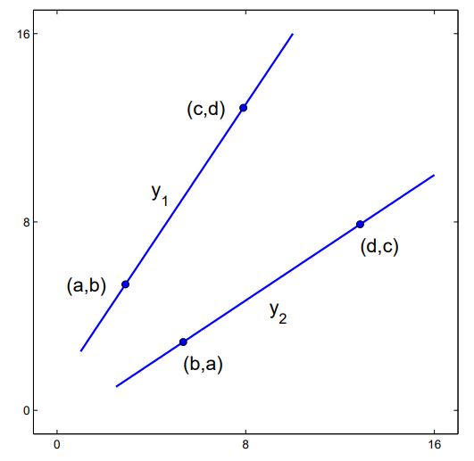
Figure \(\PageIndex{1}\): Graphs of \(y=1+(3 / 2) x\) and \(y=-2 / 3+(2 / 3) x\); each is the inverse of the other and the slopes, 3/2 and 2/3 are reciprocals.

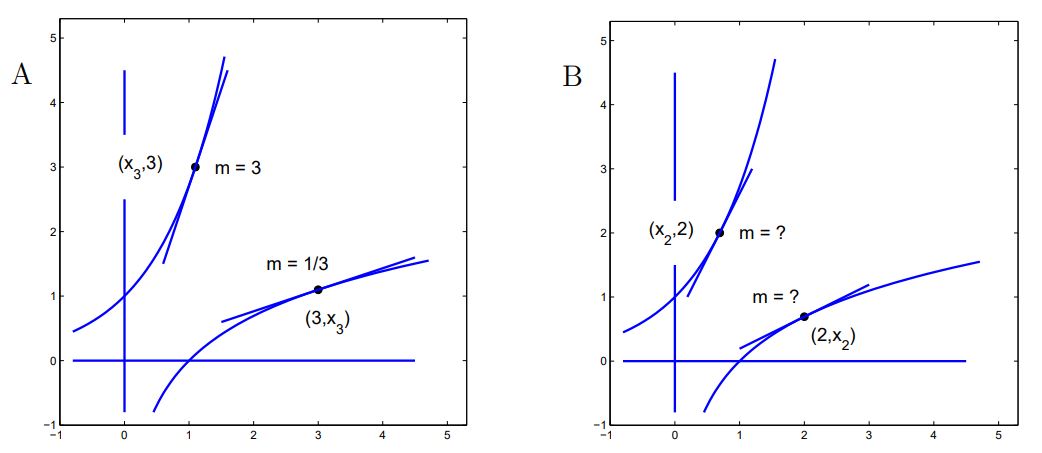
Figure \(\PageIndex{2}\): Graphs of \(E(x)=e^{x}\) and \(L(x)=\ln x\). Each is the inverse of the other. The point A has coordinates \((2, x_{2})\) and the slope of \(L\) at A is 1/2.

Explore 6.3.2

1. Evaluate \(x_3\) in Figure \(PageIndex{2}\)A.
2. Evaluate \(x_2\) in Figure \(\PageIndex{2}\)B and find the slope at \((x_{2}, 2)\) and at \((2, x_{2}) \).

The derivative of a inverse of a function.

If \(g\) is an invertible function that has a nonzero derivative and \(h\) is its inverse, then for every number, \(t\), in the domain of \(g\),

\[g^{\prime}(h(t))=\frac{1}{h^{\prime}(t)} \quad \text { and } \quad g^{\prime}(t)=\frac{1}{h^{\prime}(g(t))}\]

If \(g\) is an invertible function and \(h\) is its inverse, then for every number, \(t\), in the domain of \(g\),

\[g(h(t))=t\]

We differentiate both sides of this equation.

\[\begin{aligned}
{[g(h(t))]^{\prime} } &=[t]^{\prime} & \\
g^{\prime}(h(t)) h^{\prime}(t) &=1 & \text { Uses the Chain Rule } \\
h^{\prime}(t) &=\frac{1}{g^{\prime}(h(t))} &\text { Assumes } g^{\prime}(h(t)) \neq 0
\end{aligned}\]

Explore 6.3.3 Begin with \(h( g(t) ) = t\) and show that

\[g^{\prime}(t)=\frac{1}{h^{\prime}(g(t))}\]

Example 6.3.3 The function, \(h(t) = \sqrt{t}\), \(t > 0\) is the inverse of the function, \(g(x) = x ^{2} , ~x > 0\).

\[\begin{aligned}
g^{\prime}(x) &=2 x \\
h^{\prime}(t) &=\frac{1}{g^{\prime}(h(t))}=\frac{1}{2 h(t)}=\frac{1}{2 \sqrt{t}},
\end{aligned}\]

a result that we obtained directly from the definition of derivative.

Leibnitz notation. The Leibnitz notation for the derivative of the inverse is deceptively simple. Let \(y = g(x)\) and \(x = h(y)\) be inverses. Then \(g^{\prime}(x)=\frac{d y}{d x}\) and \(h^{\prime}(y)=\frac{d x}{d y}\). The equation

\[h^{\prime}(t)=\frac{1}{g^{\prime}(h(t))} \quad \text { becomes } \quad \frac{d x}{d y}=\frac{1}{\frac{d y}{d x}}\]

 

Exercises for Section 6.3 Derivatives of inverse functions.

Exercise 6.3.1 Find formulas for the inverses of the following functions. See Section 2.6.2 for a method. Then draw the graphs of the function and its inverse. Plot the point listed with each function and find the slope of the function at that point; plot the corresponding point of the inverse and find the slope of the inverse at that corresponding point.

1. \(P(t)=4-\frac{1}{2} t \quad 0 \leq t \leq 4 \quad(2,3)\)
2. \(P(t)=\frac{1}{1+t} \quad 0 \leq t \leq 2 \quad\left(1, \frac{1}{2}\right)\)
3. \(P(t)=\sqrt{4-t} \quad 0 \leq t \leq 4 \quad (2, \sqrt{2})\)
4. \(P(t)=2^{t} \quad 0 \leq t \leq 2 \quad (0,1)\)
5. \(P(t)=t^{2}+1 \quad-2 \leq t \leq 0 \quad(-1,2)\)
6. \(P(t)=\sqrt{4-t^{2}} \quad 0 \leq t \leq 2 \quad(1, \sqrt{3})\)

Exercise 6.3.2 The function, \(h(t) = t ^{1/3}\) is the inverse of the function \(g(x) = x ^{3}\). Use steps similar to those of Example 6.3.3 to compute \(h ^{\prime} (t)\).

Exercise 6.3.3 The graphs of a function \(F\). its inverse \(F ^{-1}\), and its derivative \(F ^{\prime}\) are shown in each of Figure 6.3.3 (a) and (b).

1. Identify each graph in Figure 6.3.3 (a) as \(F, F ^{-1}\) or \(F^{\prime}\).
2. Identify each graph in Figure 6.3.3 (b) as \(F, F ^{-1}\) or \(F^{\prime}\).

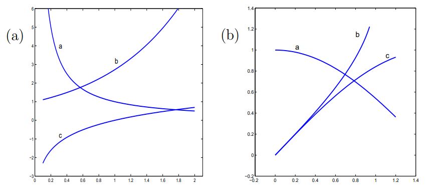
Figure for Exercise 6.3.3 Graphs of a function \(F, F ^{-1}\) or \(F^{\prime}\). See Exercise 6.3.3.