2.6: New functions from old

It is often important to recognize that a function of interest is made up of component parts — other functions that are combined to make up the function of central interest. Researchers monitoring natural populations (deer, for example) partition the dynamics into the algebraic sum of births, deaths, and harvest. Researchers monitoring annual grain production in the United States decompose the production into the product of the number of acres planted and yield per acre.

\[\text{Total Corn Production } = \text{ Acres Planted to Corn } \times \text{ Yield per Acre}\]

\[P(t)=A(t) \times Y(t)\]

Factors that influence \(A(t)\), the number of acres planted (government programs, projected corn price, alternate cropping opportunities, for example) are qualitatively different from the factors that influence \(Y(t)\), yield per acre (corn genetics, tillage practices, and weather).

 

2.6.1 Arithmetic combinations of functions.

A common mathematical strategy is “divide and conquer” — partition your problem into smaller problems, each of which you can solve. Accordingly it is helpful to recognize that a function is composed of component parts. Recognizing that a function is the sum, difference, product, or quotient of two functions is relatively simple.

Definition 2.6.1: Arithmetic Combinations of Functions.

If F and G are two functions with common domain, D, The sum, difference, product, and quotient of F and G are functions, \(F+G, F-G, F \times G\), and \(F \div G\), respectively defined by

\[\begin{aligned}
(F+G)(x) &=F(x)+G(x) & \text { for all } x \text { in } D \\
(F-G)(x) &=F(x)-G(x) & \text { for all } x \text { in } D \\
(F \times G)(x) &=F(x) \times G(x) & \text { for all } x \text { in } D \\
(F \div G)(x) &=F(x) \div G(x) & \text { for all } x \text { in } D \text { with } & G(x) \neq 0
\end{aligned}\]

For example \(F(t) = 2^{t} + t^{2}\) is the sum of an exponential function, \(E(t) = 2^t\) and a quadratic function, \(S(t) = t^2\). Which of the two functions dominates (contributes most to the value of \(F\)) for \(t < 0\)? For \(t > 0\) (careful here, the graphs are incomplete). Shown in Figure 2.6.1 are the graphs of \(E\) and \(S\).

Next in Figure 2.6.2 are the graphs of

\[E+S, \quad E-S, \quad E \times S, \quad \text { and } \quad \frac{E}{S}\]

but not necessarily in that order. Which graph depicts which of the combinations of \(S\) and \(E\)?

Figure \(\PageIndex{1}\): Graphs of A. \(E(t) = 2^t\) and B. \(S(t) = t^2\).

Figure \(\PageIndex{2}\): Graphs of the sum, difference, product, and quotient of \(E(t) = 2^t\) and \(S(t) = t^2\).

Note first that the domains of \(E\) and \(S\) are all numbers, so that the domains of \(E + S, E − S\), and \(E \times S\) are also all numbers. However, the domain of \(E/S\) excludes 0 because \(S(0) = 0\) and \(E(0)/S(0) = 1/0\) is meaningless.

The graph in Figure 2.6.2(c) appears to not have a point on the y-axis, and that is a good candidate for \(E/S\). \(E(t)\) and \(S(t)\) are never negative, and the sum, product, and quotient of non-negative numbers are all non-negative. However, the graph in Figure 2.6.2(b) has some points below the x-axis, and that is a good candidate for \(E − S\).

The product, \(E \times S\) is interesting for \(t < 0\). The graph of \(E = 2^t\) is asymptotic to the negative t-axis; as t progresses from -1 to -2 to -3 to \(\cdots , E(t)\) is \(2^{−1} = 0.5, 2^{−2} = 0.25, 2^{−3} = 0.125, \cdots\) and gets close to zero. But \(S(t) = t^2\) is \((−1)^{2} = 1, (−2)^{2} = 3, (−3)^{2} = 9, \cdots\) gets very large. What does the product do?

 

2.6.2 The inverse of a function.

Suppose you have a travel itinerary as shown in Table 2.5. If your traveling companion asks,

Table 2.5: Itinerary for (brief) European trip.

Day	June 1	June 2	June 3	June 4	June 5	June 6	June 7
City	London	London	London	Brussels	Paris	Paris	Paris

“What day were we in Brussels?”, you may read the itinerary ‘backward’ and respond that you were in Brussels on June 4. On the other hand, if your companion asks, “I cashed a check in Paris, what day was it?”, you may have difficulty in giving an answer.

An itinerary is a function that specifies that on day, \(x\), you will be in location, \(y\). You have inverted the itinerary and reasoned that the for the city Brussels, the day was June 4. Because you were in Paris June 5 - 7, you can not specify the day that the check was cashed.

Charles Darwin exercised an inverse in an astounding way. In his book, On the Various Contrivances by which British and Foreign Orchids are Fertilised by Insects he stated that the angraecoids were pollinated by specific insects. He noted that A. sesquipedale in Madagascar had nectaries eleven and a half inches long with only the lower one and one-half inch filled with nectar. He suggested the existence of a ’huge moth, with a wonderfully long proboscis’ and noted that if the moth ’were to become extinct in Madagascar, assuredly the Angraecum would become extinct.’ Forty one years later Xanthopan morgani praedicta was found in tropical Africa with a proboscis of ten inches.

Such inverted reasoning occurs often.

Explore 2.6.1 Answer each of the following by examining the inverse of the function described.

1. Rate of heart beat increases with level of exertion; heart is beating at 165 beats per minute; is the level of exertion high or low? You may want to visit en.wikipedia.org/wiki/Heart_rate.
2. Resting blood pressure goes up with artery blockage; resting blood pressure is 110 (systolic) ‘over’ 70 (diastolic); is the level of artery blockage high or low? The answer can be found in en.wikipedia.org/wiki/Blood_Pressure.
3. Diseases have symptoms; a child is observed with a rash over her body. Is the disease chicken pox?

The child with a rash in Example c. illustrates again an ambiguity often encountered with inversion of a function; the child may in fact have measles and not chicken pox. The inverse information may be multivalued and therefore not a function. Nevertheless, the doctor may make a diagnosis as the most probable disease, given the observed symptoms. She may be influenced by facts such as

• Blood analysis has demonstrated that five other children in her clinic have had chicken pox that week and
• Because of measles immunization, measles is very rare.

It may be that she can actually distinguish chicken pox rash from measles rash, in which case the ambiguity disappears.

The definition of the inverse of a function is most easily made in terms of the ordered pair definition of a function. Recall that a function is a collection of ordered number pairs, no two of which have the same first term.

Definition 2.6.2: Inverse of a Function.

A function F is invertible if no two ordered pairs of F have the same second number. The inverse of an invertible function, F, is the function G to which the ordered pair (x,y) belongs if and only if (y,x) is an ordered pair of F. The function, G, is often denoted by \(F^{−1}\).

Explore 2.6.2 Do This. Suppose G is the inverse of an invertible function F. What is the inverse of G?

Table 2.6: Of the two itineraries shown below, the one on the left is invertible.

Day Location Day Location June 4 London June 8 Vienna June 5 Amsterdam June 9 Zurich June 6 Paris June 10 Venice June 7 Berlin June 11 Rome

Day Location Day Location June 4 London June 8 Zurich June 5 Paris June 9 Zurich June 6 Paris June 10 Rome June 7 Paris June 11 Rom

The notation \(F^{−1}\) for the inverse of a function \(F\) is distinct from the use of −1 as an exponent meaning division, as in \(2^{−1} = \frac{1}{2}\). In this context, \(F^{−1}\) does not mean \frac{1}{F} , even though students have good reason to think so from previous use of the symbol, −1 . The TI-86 calculator (and others) have keys marked \(\sin ^{−1}\) and \(x^{−1}\). In the first case, the −1 signals the inverse function, \(\arcsin{x}\), in the second case the −1 signals reciprocal, \(1/x\). Given our desire for uniqueness of definition and notation, the ambiguity is unfortunate and a bit ironic. There is some recovery, however. You will see later that the composition of functions has an algebra somewhat like ‘multiplication’ and that ‘multiplying’ by an inverse of a function \(F\) has some similarity to ‘dividing’ by \(F\). At this stage, however, the only advice we have is to interpret \(h^{−1}\) as ‘divide by \(h\)’ if \(h\) is a number and as ‘inverse of \(h\)’ if \(h\) is a function or a graph.

The graph of a function easily reveals whether it is invertible. Remember that the graph of a function is a simple graph, meaning that no vertical line contains two points of the graph.

Definition 2.6.3: Invertible Graph.

An invertible simple graph is a simple graph for which no horizontal line contains two points. A simple graph is invertible if and only if it is the graph of an invertible function.

The simple graph G in Figure 2.6.3(a) has two points on the same horizontal line. The points have the same y-coordinate, \(y_1\), and thus the function defining G has two ordered pairs, (\(x_{1}, y_{1}\)) and (\(x_{2}, y_{1}\)) with the same second term. The function is not invertible. The same simple graph G does contain a simple graph that is invertible, as shown as the solid curve in Figure 2.6.3(b), and it is maximal in the sense that if any additional point of the graph of G is added to it, the resulting graph is not invertible.

Figure \(\PageIndex{3}\): Graph of a function that is not invertible.

Explore 2.6.3 Find another simple graph contained in the graph G of Figure 2.6.3(a) that is invertible. Is your graph maximal? Is there a simple graph contained in G other than that shown in Figure 2.6.3 that is invertible and maximal?

Example 2.6.1 Shown in Figure 2.6.4 is the graph of an invertible function, \(F\), as a solid line and the graph of \(F^{−1}\) as a dashed line. Tables of seven ordered pairs of \(F\) and seven ordered pairs of \(F^{−1}\) are given. Corresponding to the point, \(P (3.0, 1.4)\) of \(F\) is the point, \(Q (1.4, 3.0)\) of \(F^{−1}\). The line \(y = x\) is the perpendicular bisector of the interval, \(\overline{P Q}\). Observe that the domain of \(F^{−1}\) is the range of F, and the range of \(F^{−1}\) is the domain of \(F\).

The preceding example lends support for the following observation.

The graph of the inverse of \(F\) is the reflection of the graph of \(F\) about the diagonal line, \(y = x\).

The reflection of G with respect to the diagonal line, \(y = x\) consists of the points \(Q\) such that either \(Q\) is a point of \(G\) on the diagonal line, or there is a point \(P\) of \(G\) such that the diagonal line is the perpendicular bisector of the interval \(\overline{P Q}\).

The concept of the inverse of a function makes it easier to understand logarithms. Shown in Table 2.7 are some ordered pairs of the exponential function, \(F(x) = 10^x\) and some ordered pairs of the logarithm function \(G(x)=\log _{10}(x)\). The logarithm function is simply the inverse of the exponential function.

\(F\)		\(F^{-1}\)
1.0	0.200	0.200	1.0
1.5	0.575	0.575	1.5
2.0	0.800	0.800	2.0
2.5	1.025	1.025	2.5
3.0	1.400	1.400	3.0
3.5	2.075	2.075	3.5
4.0	3.200	3.200	4.0

Figure \(\PageIndex{4}\): Graph of a function \(F\) (solid line) and its inverse \(F^{−1}\) (dashed line) and tables of data for \(F\) and \(F^{−1}\).

 

Table 2.7: Partial data for the function \(F(x) = 10^x\) and its inverse \(G(x) = \log_{10} (x)\).

\(x\)	\(10^x\)	\(x\)	\(\log_{10} x\)
-2	0.01	0.01	-2
-1	0.1	0.1	-1
0	1	1	0
1	10	10	1
2	100	100	2
3	1000	1000	3

 

The function \(F(x) = x^2\) is not invertible. In Figure 2.6.5 both (-2,4) and (2,4) are points of the graph of \(F\) so that the horizontal line \(y = 4\) contains two points of the graph of \(F\). However, the function \(S\) defined by

\[S(x)=x^{2} \quad \text { for } x \geq 0\]

is invertible and its inverse is

\[S^{-1}(x)=\sqrt{x}\]

 

2.6.3 Finding the equation of the inverse of a function.

There is a straightforward means of computing the equation of the inverse of a function from the equation of the function. The inverse function reverses the role of the independent and dependent variables. The independent variable for the function is the dependent variable for the inverse function. To compute the equation for the inverse function, it is common to interchange the symbols for the dependent and independent variables.

Example 2.6.2 To compute the equation for the inverse of the function S,

\[S(x)=x^{2} \quad \text { for } \quad x \geq 0\]

Figure \(\PageIndex{5}\): Graph of \(F(x) = x^2\); (-2,4) and (2,4) are both points of the graph indicating that \(F\) is not invertible.

let the equation for S be written as

\[y=x^{2} \quad \text { for } \quad x \geq 0\]

Then interchange y and x to obtain

\[x=y^{2} \quad \text { for } \quad y \geq 0\]

and solve for y.

\[\begin{aligned}
x &=y^{2} \quad \text { for } \quad y \geq 0 \\
y^{2} &=x \quad \text { for } \quad y \geq 0 \\
\left(y^{2}\right)^{\frac{1}{2}} &=x^{\frac{1}{2}} \\
y^{2 \frac{1}{2}} &=x^{\frac{1}{2}} \\
y &=x^{\frac{1}{2}}
\end{aligned}\]

Therefore

\[S^{-1}(x)=\sqrt{x} \quad \text { for } \quad x \geq 0\]

Example 2.6.3 The graph of function \(F(x) = 2x^{2} − 6x + 3/2\) shown in Figure 2.6.6 has two invertible portions, the left branch and the right branch. We compute the inverse of each of them. Let \(y = 2x^{2} − 6x + 5/2\), exchange symbols \(x = 2y^{2} − 6y + 5/2\), and solve for \(y\). We use the steps of ‘completing the square’ that are used to obtain the quadratic formula.

Figure \(\PageIndex{6}\): Graph of \(F(x) = 2x^{2} − 6x + 3/2\) showing the left branch as dashed line and right branch as solid line.

steps of ‘completing the square’ that are used to obtain the quadratic formula.

\[\begin{aligned}
x &=2 y^{2}-6 y+5 / 2 \\
&=2\left(y^{2}-3 x+9 / 4\right)-9 / 2+5 / 2 \\
&=2(y-3 / 2)^{2}-2 \\
(y-3 / 2)^{2} &=\frac{x+2}{2} \\
y-3 / 2 &=\sqrt{\frac{x+2}{2}} \text { or } \quad-\sqrt{\frac{x+2}{2}} \\
y &=\frac{3}{2}+\sqrt{\frac{x+2}{2}} & \text { Right branch inverse. } \\
y &=\frac{3}{2}-\sqrt{\frac{x+2}{2}} & \text { Left branch inverse. }
\end{aligned}\]

 

Exercises for Section 2.6 New functions from old.

Exercise 2.6.1 In Figure 2.6.2 identify the graphs of \(E + S\) and \(E \times S\).

Exercise 2.6.2 Three examples of biological functions and questions of inverse are described in Explore 2.6.1. Identify two more functions and related inverse questions.

Exercise 2.6.3 The genetic code appears in Figure 2.2.2. It occasionally occurs that the amino acid sequence of a protein is known, and one wishes to know the DNA sequence that coded for it. That the genetic code is not invertible is illustrated by the following problem.

Find two DNA sequences that code for the amino acid sequence KYLEF. (Note: K = Lys = lysine, Y = Tyr = tyrosine, L = Leu = leucine, E = Glu = glutamic acid, F = Phe = phenylalanine. The sequence KYLEF occurs in sperm whale myoglobin.)

Exercise 2.6.4 Which of the following functions are invertible?

1. The distance a DNA molecule will migrate during agarose gel electrophoresis as a function of the molecular weight of the molecule, for domain: \(1kb \leq \text{ Number of bases } \leq 20kb\).
2. The density of water as a function of temperature.
3. Day length as a function of elevation of the sun above the horizon (at, say, 40 degrees North latitude).
4. Day length as a function of day of the year.

Exercise 2.6.5 Shown in Figure Ex. 2.6.5 is the graph of a function, \(F\). Some ordered pairs of the function are listed in the table and plotted as filled circles. What are the corresponding ordered pairs of \(F^{−1}\)? Plot those points and draw the graph of \(F^{−1}\).

\(x\)	\(F(x)\)
0	0
1	0.2
2	0.8
3	1.8
4	3.2
5	1.0
6	7.2

Figure for Exercise 2.6.5 Partial data and a graph of an invertible function, \(F\), and the diagonal, \(y = x\). See Exercise 2.6.5.

Exercise 2.6.6 Shown in Figure Ex. 2.6.6 is the graph of \(F(x) = 2^x\). (-2,1/4), (0,1), and (2,4) are ordered pairs of \(F\). What are the corresponding ordered pairs of \(F^{−1}\)? Plot those points and draw the graph of \(F^{−1}\).

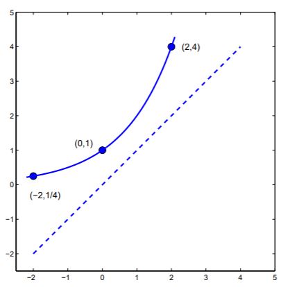
Figure for Exercise 2.6.6 Graph of \(F(x) = 2^x\) and the diagonal, \(y = x\). See Exercise 2.6.6

Exercise 2.6.7 In Subsection 2.2.2 Simple Graphs and Figure 2.2.1 it is observed that the circle is not a simple graph but contained several simple graphs that were ‘as large as possible’, meaning that if another point of the circle were added to them they would not be simple graphs. Neither of the examples in Figure 2.2.1 is invertible. Does the circle contain a simple graph that is as large as possible and that is an invertible simple graph?

Exercise 2.6.8 Shown in Figure Ex. 2.6.8 is a graph of a function, \(F\). Make a table of \(F\) and \(F^{−1}\) and plot the points of the inverse. Let \(G\) be \(F^{−1}\) . Make a table of \(G^{−1}\) and plot the points of \(G^{−1}\).

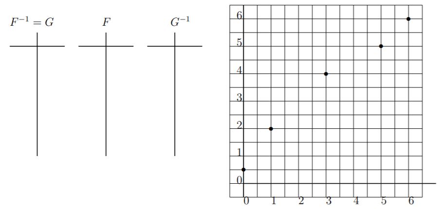
Figure for Exercise 2.6.8 Graph of a function \(F\). See Exercise 2.6.8.

Exercise 2.6.9 Is there an invertible function whose domain is the set of positive numbers and whose range is the set of non-negative numbers?

Exercise 2.6.10 Incredible! Find the inverse of the function, \(F\), defined by

Hint: Look at its graph.

Exercise 2.6.11 Answer the question in Explore 2.6.2, Suppose \(G\) is the inverse of an invertible function \(F\). What is the inverse of \(G\)?

Exercise 2.6.12 Find equations for the inverses of the functions defined by

1. \(F_{1}(x)=\frac{1}{x+1}\)
2. \(F_{2}(x)=\frac{x}{x+1}\)
3. \(F_{3}(x)=1+2^{x}\)
4. \(F_{4}(x)=\log _{2} x-\log _{2}(x+1)\)
5. \(F_{5}(x)=10^{-x^{2}} \text{ for } x \geq 0\)
6. \(F_{6}(z)=\frac{z+\frac{1}{z}}{2} \text{ for } z \geq 1\)
7. \(F_{7}(x)=\frac{2^{x}-2^{-x}}{2}\)

Hint for (g): Let \(y = \frac{2^{x}−2^{−x}}{2}\), interchange \(x\) and \(y\) so that \(x = \frac{2^{y}−2^{−y}}{2} , then substitute \(z = 2^y\) and solve for \(z\) in terms of \(x\). Then insert \(2^{y} = z\) and solve for \(y\).

Exercise 2.6.13 Mutations in mitochondrial DNA occur at the rate of 15 per \(10^2\) base pairs per million years. Therefore, the number of differences, \(D\), expected between two present mitochondrial DNA sequences of length \(L\) would be

\[D=2 \frac{15}{100} L \frac{T}{1000000} \label{2.8}\]

where T is number of years since the most recent ancestor of the mitochondrial sequences.

1. Explain the factor of 2 in Equation \ref{2.8}. (Hint: consider the phylogenetic tree shown in Figure Ex. 2.6.13)
2. The African pygmy and the Papua-New Guinea aborigine mitochondrial DNA differ by 2.9%. How many years ago did their ancestral populations diverge?

Figure for Exercise 2.6.13 Phylogenetic tree showing divergence from an ancestor.