2.5: Least squares fit of polynomials to data

Last updated
Save as PDF

Page ID: 36842

$ \newcommand{\vecs}[1]{\overset { \scriptstyle \rightharpoonup} {\mathbf{#1}} } $ $ \newcommand{\vecd}[1]{\overset{-\!-\!\rightharpoonup}{\vphantom{a}\smash {#1}}} $$\newcommand{\id}{\mathrm{id}}$ $ \newcommand{\Span}{\mathrm{span}}$ $ \newcommand{\kernel}{\mathrm{null}\,}$ $ \newcommand{\range}{\mathrm{range}\,}$ $ \newcommand{\RealPart}{\mathrm{Re}}$ $ \newcommand{\ImaginaryPart}{\mathrm{Im}}$ $ \newcommand{\Argument}{\mathrm{Arg}}$ $ \newcommand{\norm}[1]{\| #1 \|}$ $ \newcommand{\inner}[2]{\langle #1, #2 \rangle}$ $ \newcommand{\Span}{\mathrm{span}}$ $\newcommand{\id}{\mathrm{id}}$ $ \newcommand{\Span}{\mathrm{span}}$ $ \newcommand{\kernel}{\mathrm{null}\,}$ $ \newcommand{\range}{\mathrm{range}\,}$ $ \newcommand{\RealPart}{\mathrm{Re}}$ $ \newcommand{\ImaginaryPart}{\mathrm{Im}}$ $ \newcommand{\Argument}{\mathrm{Arg}}$ $ \newcommand{\norm}[1]{\| #1 \|}$ $ \newcommand{\inner}[2]{\langle #1, #2 \rangle}$ $ \newcommand{\Span}{\mathrm{span}}$$\newcommand{\AA}{\unicode[.8,0]{x212B}}$

Polynomials and especially linear functions are often ’fit’ to data as a means of obtaining a brief and concise description of the data. The most common and widely used method is the method of least squares. To fit a line to a data set, $(x_{1}, y_{1}), (x_{2}, y_{2}), \cdots (x_{n}, y_{n})$, one selects $a$ and $b$ that minimizes

\[\sum_{k=1}^{n}\left(y_{k}-a-b x_{k}\right)^{2} \label{2.2}\]

$2-5.JPG$

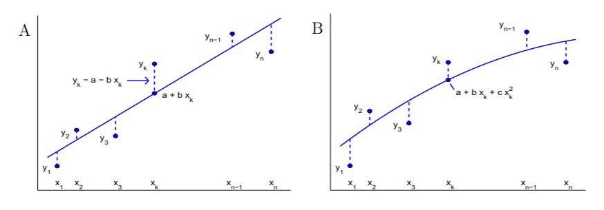
Figure $\PageIndex{1}$: A. Least squares fit of a line to data. B. Least squares fit of a parabola to data.

The geometry of this equation is illustrated in Figure 2.5.1. The goal is to select $a$ and $b$ so that the sum of the squares of the lengths of the dashed lines is as small as possible. We show in in Example 13.2.2 that the optimum values of $a$ and $b$ satisfy

\[\begin{array}\\
a n+b \sum_{k=1}^{n} x_{k} &=\sum_{k=1}^{n} y_{k} \\
a \sum_{k=1}^{n} x_{k}+ b \sum_{k=1}^{n} x_{k}^{2} &=\sum_{k=1}^{n} x_{k} y_{k}
\end{array} \label{2.3}\]

**Table 2.2:** Relation between temperature and frequency of cricket chirps.
Temperature ($^{\circ} F$)
Chirps per Minute	109	136	160	87	103	102	108	154	144	150

The solution to these equations is

\[\begin{array}\\
a \quad =& \quad \frac{\sum_{k=1}^{n} x_{k}^{2} \sum_{k=1}^{n} y_{k}-\left(\sum_{k=1}^{n} x_{k}\right)\left(\sum_{k=1}^{n} x_{k} y_{k}\right)}{\Delta} \\
b \quad =& \quad \frac{n \sum_{k=1}^{n} x_{k} y_{k}-\left(\sum_{k=1}^{n} x_{k}\right)\left(\sum_{k=1}^{n} y_{k}\right)}{\Delta} \\
\Delta \quad =& \quad n \sum_{k=1}^{n} x_{k}^{2}-\left(\sum_{k=1}^{n} x_{k}\right)^{2}
\end{array} \label{2.4}\]

Example 2.5.1 If we use these equations to fit a line to the cricket data of Example 1.10.1 showing a relation between temperature and cricket chirp frequency, we get

\[y=4.5008 x-192.008 \quad \text{ close to the line } \quad y=4.5 x-192\]

that we ’fit by eye’ using the two points, (65,100) and (75,145).

Explore 2.5.1 Technology. Your calculator or computer will hide all of the arithmetic of Equations \ref{2.4} and give you the answer. The overall procedure is:

Load the data. [Two lists, X and Y, say].
Compute the coefficients of a first degree polynomial close to the data and store them in P.
Specify X coordinates and compute corresponding Y coordinates for the polynomial.
Plot the original data and the computed polynomial.

A MATLAB program to do this is:

Code $\PageIndex{1}$ (MATLAB):

close all;clc;clear

X=[67 73 78 61 66 66 67 77 74 76];

Y=[109 136 160 87 103 102 108 154 144 150];

P=polyfit(X,Y,1)

PX=[60:0.1:80];

PY=polyval(P,PX);

plot(X,Y,’+’,’linewidth’,2); hold(’on’); plot(PX,PY,’linewidth’,2)

**Table 2.3:** A tube is filled with water and a hole is opened at the bottom of the tube. Relation between height of water remaining in the tube and time.
Time (sec)	0	5	10	15	20	25	30	35	40	45	50	55	60
Height (cm)	85	73	63	54	45	36	29	22	17	12	7	4	2

To fit a parabola to a data set, $(x_{1}, y_{1}), (x_{2}, y_{2}), \cdots (x_{n}, y_{n})$, one selects $a, b$ and $c$ that minimizes

\[\sum_{k=1}^{n}\left(y_{k}-a-b x_{k}-c x_{k}^{2}\right)^{2} \label{2.5}\]

The geometry of this equation is illustrated in Figure 2.5.1B. The goal is to select $a, b$ and $c$ so that the sum of the squares of the lengths of the dashed lines is as small as possible. The optimum values of $a, b$, and $c$ satisfy (Exercise 14.2.4)

\[\begin{array}\\
a n+b \sum x_{k}+c \sum x_{k}^{2} &=\sum y_{k} \\
a \sum x_{k}+b \sum x_{k}^{2}+c \sum x_{k}^{3} &=\sum x_{k} y_{k} \\
a \sum x_{k}^{2}+b \sum x_{k}^{3}+c \sum x_{k}^{4} &=\sum x_{k}^{2} y_{k}
\end{array} \label{2.6}\]

There is a methodical procedure for solving three linear equations three variables using pencil and paper. For now it is best to rely on your calculator or computer.

Explore 2.5.2 Technology. Fit a parabola to the water draining from a tube data of Figure 1.10.2 reproduced in Table 2.3.

The procedure will be almost identical to that of Explore 2.5.1. The difference is that in step 2 you will compute the coefficients of a second degree polynomial. The line P=polyfit(X,Y,1) will be changed to P=polyfit(X,Y,2) . In the program, of course, the data will be different and the PX-values for the polynomial will be adjusted to the data.

Example 2.5.2 A graph of the polio data from Example 2.2.1 showing the percent of U.S. population that had antibodies to the polio virus in 1955 is shown in Figure 2.5.2. Also shown is a graph of the fourth degree polynomial

\[P_{4}(x)=-4.13+7.57 x-0.136 x^{2}-0.00621 x^{3}+0.000201 x^{4}\]

The polynomial that ‘fit’ the polio data using a MATLAB program similar to that described in Explore 2.5.1 and discussed in Explore 2.5.2 The technology selects the coefficients, $-4.14, 7.57, \cdots$ so that the sum of the squares of the distances from the polynomial to the data is as small as possible.

$2-6.JPG$

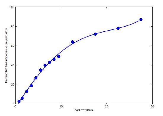
Figure $\PageIndex{2}$: A fourth-degree polynomial fit to data for percent of people in 1955 who had antibodies to the polio virus as a function of age. Data read from Anderson and May, Vaccination and herd immunity to infectious diseases, Nature 318 1985, pp 323-9, Figure 2f.

Exercises for Section 2.5, Least squares fit of polynomials to data.

Exercise 2.5.1 Use Equations 2.3 to find the linear function that is the least squares fit to the data:

\[(-2,5) \quad(3,12)\]

Exercise 2.5.2 Use Equations 2.6 to find the quadratic function that is the least squares fit to the data:

\[(-2,5) \quad(3,12) \quad(10,0)\]

Exercise 2.5.3 Technology Shown in the Table 2.4 are the densities of water at temperatures from 0 to 100 $^{\circ} C$ Use your calculator or computer to fit a cubic polynomial to the data. See Explore 2.5.1 and Explore 2.5.2. Compare the graphs of the data and of the cubic.

**Table 2.4:** The density of water at various temperatures Source: Robert C. Weast, Melvin J. Astle, and William H. Beyer, *CRC Handbook of Chemistry and Physics*, 68th Edition, 1988, CRC Press, Boca Raton, FL, p F-10.
Temp ($^{\circ} C$)	Density ($g/cm^3$)	Temp ($^{\circ} C$)	Density ($g/cm^3$)
0	0.99987	45	0.99025
3.98	1.00000	50	0.98807
5	0.99999	55	0.98573
10	0.99973	60	0.98324
15	0.99913	65	0.98059
18	0.99862	70	0.97781
20	0.99823	75	0.97489
25	0.99707	80	0.97183
30	0.99567	85	0.96865
35	0.99406	90	0.96534
38	0.99299	95	0.96192
40	0.99224	100	0.95838

$tbl2-4.JPG$

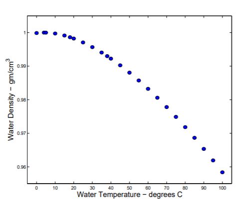
Exercise 2.5.3 $D(T)=1.00004105+0.00001627 T-0.000005850 T^{2}+0.000000015324 T^{3}$

Temperature (\(^{\circ} F\))
Chirps per Minute	109	136	160	87	103	102	108	154	144	150