1.10: Data modeling vs mathematical models.

In Example 1.9.1 of light intensity from a 12 volt bulb we modeled data and only subsequently built a mathematical model of light decrease from a point source of light. There are other examples of modeling of data that are interesting but there is very little possibility of building a mathematical model to explain the process. See Also: mathinsight.org/data_modeling...tical_modeling

Example 1.10.1 Jack A. Wolfe¹⁴ observed that leaves of trees growing in cold climates tend to be incised (have ragged edges) and leaves of trees growing in warm climates tend to have smooth edges (lacking lobes or teeth). He measured the percentages of species that have smooth margins among all species of the flora in many locations in eastern Asia. His data, as read from a graph in U. S. Geological Survey Professional Paper 1106, is presented in Figure 1.10.0.2.

Figure for Example 1.10.0.2 Average temperature \(C^{\circ}\) vs percentage of tree species with smooth edge leaves in 33 forests in eastern Asia. The equation of the line is \(y = −0.89 + 0.313x\).

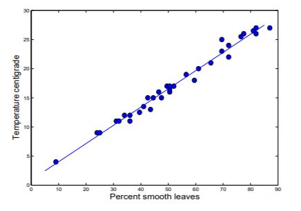
The line, temp = 0.89 + 0.313 % smooth is shown in Figure 1.10.0.2 and is close to the data. The line was used by Wolfe to estimate temperatures over the last 65 million years based on observed fossil leaf composition (Exercise 1.10.1). The prospects of writing a mathematical model describing the relationship of smooth edge leaves to temperature are slim, however.

Example 1.10.1 On several nights during August and September in Ames, Iowa, some students listened to crickets chirping. They counted the number of chirps in a minute (chirp rate, \(R\)) and also recorded the air (ambient) temperature (T) in \(F^{\circ}\) for the night. The data were collected between 9:30 and 10:00 pm each night, and are shown in the table and graph in Figure 1.24.

Temperature (\(^{\circ} F\)) \(T\)	Chirps per Minute \(R\)
67	109
73	136
78	160
61	87
66	103
66	102
67	108
77	154
74	144
76	150

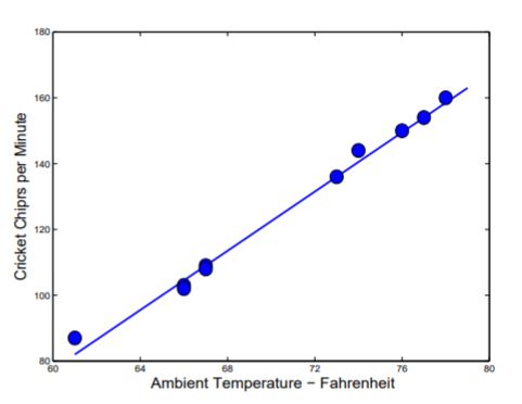
Figure \(\PageIndex{1}\): A table and graph of the frequency of cricket chirps vs temperature in degrees \(F^{\circ}\).

These data also appear linear and the line through (65,100) and (75,145),

\[\frac{R-100}{T-65}=\frac{145-100}{75-65}, \quad R=4.5 T-192.5 \label{1.32}\]

lies close to the data. We can use the line to estimate temperature to be about 69.5 \(F^{\circ}\) if cricket chirp rate is 120 chirps/minute.

This observation was made by Amos Dolbear in 1897, see National Geographic July 2012, 222 (1), p 17 ff.

Both of these examples are examples of data modeling. We fit a line to the data, but there is no underlying explanation of what mechanism is causing the relation.

Exercises for Section 1.10, Data modeling vs mathematical models.

Exercise 1.10.1 Jack Wolfe applied his data (Figure 1.10.0.2) to resolve a dispute about estimates of ambient temperatures during the last 65 million years. Fossil leaves from strata ranging in age back to 65 million years were examined for the percent of smooth-leafed species in each stratum. Under the hypothesis that the relation between percent of smooth-leafed species and temperature in modern species persisted over the last 65 million years, he was able to estimate the past temperatures. Your job is to replicate his work. Although Wolfe collected fossil leaf data from four locations ranging from southern Alaska to Mississippi, we show only his data from the Pacific Northwest, in Table Ex. 1.10.1, read from a graph in Wolfe’s article in American Scientist 1979, 66:694-703.

Use the Percent Smooth data for the fossil leaves at previous times in Table Ex. 1.10.1, and the modern relation, temp = 0.89 + 0.313 % smooth, to draw a graph showing the history of ambient temperature for the land of the Pacific Northwest

1. Over the period from 50 to 40 million years ago.
2. Over the period from 35 to 26 million years ago.
3. Over the period from 26 to 16 million years ago.
4. Over the period from 16 to 6 million years ago.

Table for Exercise 1.10.1 Percentages of smooth-leafed species found in geological strata in the Pacific Northwest.

Age Myr	Percent Smooth	Age Myr	Percent Smooth	Age Myr	Percent Smooth	Age Myr	Percent Smooth
50	57	35	66	26	42	10	28
48	50	35	68	21	24	10	30
48	51	33	55	21	28	10	32
44	70	31	24	21	32	6	34
44	74	31	32	16	31	6	38
40	40	26	32	16	34
40	44	26	40	16	38

Exercise 1.10.2

1. Use the graph in Figure 1.24 to estimate the expected temperature if the cricket chirp rate were were 95 chirps per minute? Also use Equation \ref{1.32} to compute the same temperature and compare your results.
2. On the basis of Equation \ref{1.32}, what cricket chirp frequencies might be expected for the temperatures 110 \(^{\circ} F\) and 40 \(^{\circ} F\)? Discuss your answers in terms of the data in Figure 1.10.1 and the interval on which the equation is valid.
3. A television report stated that in order to tell the temperature, count the number of cricket chirps in 13 seconds and add 40. The result will be the temperature in Fahrenheit degrees. Is that consistent with Equation \ref{1.32}? (Suggestion: Solve for Temperature \(^{\circ} F\) in terms of Cricket Chirps per Minute.)

Exercise 1.10.3 Some students made a small hole near the bottom of the cylindrical section of a two-liter plastic beverage container, held a finger over the hole and filled the container with water to the top of the cylindrical section, at 15.3 cm. The small hole was uncovered and the students marked the height of the water remaining in the tube, reported here at eighty-second intervals, until the water ran out. They then measured the heights of the marks above the hole. The data gathered and a graph of the data are shown in Figure 1.10.2.

1. Select a curve and fit an equation for the curve to the data in Figure 1.10.2.
2. Search your physics book for a mathematical model that explains the data. A fluid dynamicist named Evangelista Torricelli (1608-1649) provided such a model (and also invented the mercury thermometer).
3. The basic idea of Torricelli’s formula is that the potential energy of a thin layer of liquid at the top of the column is converted to kinetic energy of fluid flowing out of the hole. Let the time index, \(t_{0}, t_{1}, \cdots\) measure minutes and \(h_k\) be the height of the water at time \(t_k\). The layer between \(h_k\) and \(h_{k+1}\) has mass mk and potential energy \(m_{k}gh_{k}\). During the \(k^{th}\) minute an equal mass and volume of water flows out of the hole with velocity, \(v_k\), and kinetic energy \(\frac{1}{2}m_{k}v_{k}^{2}\) . Equating potential and kinetic energies, \[m_{k} g h_{k}=\frac{1}{2} m_{k} v_{k}^{2}, \quad g h_{k}=\frac{1}{2} v_{k}^{2}\] Let \(A_{\text{cylinder}}\) and \(A_{\text{hole}\) be the cross-sectional areas of the cylinder and hole, respectively.
   1. Argue that \[v_{k}=\frac{A_{\text {cylinder }}}{A_{\text {hole }}} \frac{h_{k}-h_{k+1}}{t_{k+1}-t_{k}}=\frac{A_{\text {cylinder }}}{A_{\text {hole }}}\left(h_{k}-h_{k+1}\right)\]
   2. Argue that \[h_{k+1}=h_{k}-K \sqrt{h_{k}} \label{1.33}\] where K is a constant.
   3. Compare Equation \ref{1.33} with Equation 1.5.5.

Time (sec)	Height (cm)
0	15.3
80	12.6
160	9.9
240	7.8
320	6.2
400	4.3
480	3.1
560	2.0

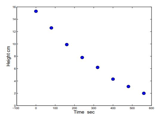
Figure \(\PageIndex{2}\): Height of water draining from a 2-liter beverage container measured at 40 second intervals.

 

¹⁴ Jack A. Wolfe, A paleobotanical interpretation of tertiary climates in northern hemisphere, American Scientist 66 (1979), 694-703