1.11: Summary

You have begun one of the most important activities in science, the writing of mathematical models. The best models are sufficiently detailed in their description that dynamic equations describing the progress of the underlying system can be written and lead to solution equations that describe the overall behavior. In our models there was a quantity (\(Q\)) that changed with either time or distance (\(v\)) and the dynamic equation specified how the change in \(Q, Q_{v+1} − Q_{v},\) depended on \(Q\) or \(v\). The solution equation explicitly expressed the relation of \(Q\) to \(v\).

In some cases, such as the case of cricket chirp frequency dependence on ambient temperature in Example 1.10.1, the underlying mechanism is too complex to model it. The observation, however, stimulates considerable thought about why it should be. Presumably the metabolism of the cricket increases with temperature thus causing an increase in chirp frequency, but the phrase, ‘metabolism of the cricket’, masks a large complexity.

We have generally followed certain steps in developing our models. They are useful steps but by no means do they capture the way to model the biological universe. The modeling process is varied and has to be adapted to the questions at hand.

By the methods of this chapter you can solve every first order linear finite difference equation with constant coefficients:

\[y_{0} \text{ given }, \quad y_{t+1} − y_{t} = r y_{t} + b \label{1.34}\]

The solution is

\[y_{t}=-\frac{b}{r}+\left(y_{0}+\frac{b}{r}\right)(r+1)^{t} \quad \text { if } \quad r \neq 0, \quad \text { or } \quad y_{t}=y_{0}+t b \quad \text { if } \quad r=0\]

Exercises for Chapter 1, Mathematical Models of Biological Processes.

Chapter Exercise 1.11.1 Two kilos of a fish poison, rotenone, are mixed into a lake which has a volume of \(100 \times 20 \times 2 = 4000\) cubic meters. No water flows into or out of the lake. Fifteen percent of the rotenone decomposes each day.

1. Write a mathematical model that describes the daily change in the amount of rotenone in the lake.
2. Let \(R_{0}, P_{1}, R_{2}, \cdots\) denote the amounts of rotenone in the lake, \(P_t\) being the amount of poison in the lake at the beginning of the \(t^{th}\) day after the rotenone is administered. Write a dynamic equation representative of the mathematical model.
3. What is \(R_0\)? Compute \(R_1\) from your dynamic equation. Compute \(R_2 \)from your dynamic equation.
4. Find a solution equation for your dynamic equation.

Note: Rotenone is extracted from the roots of tropical plants and in addition to its use in killing fish populations is used as a insecticide on such plants as tomatoes, pears, apples, roses, and African violets. Studies in which large amounts (2 to 3 mg/Kg body weight) of rotenone were injected into the jugular veins of laboratory rats produced symptoms of Parkinson’s disease, including the reduction of dopamine producing cells in the brain. (Benoit I. Giasson & Virginia M.-Y. Lee, A new link between pesticides and Parkinson’s disease, Nature Neuroscience 3, 1227 - 1228 (2000)).

Chapter Exercise 1.11.2 Two kilos of a fish poison that does not decompose are mixed into a lake that has a volume of \(100 \times 20 \times 2 = 4000\) cubic meters. A stream of clean water flows into the lake at a rate of 1000 cubic meters per day. Assume that it mixes immediately throughout the whole lake. Another stream flows out of the lake at a rate of 1000 cubic meters per day.

1. Write a mathematical model that describes the daily change in the amount of poison in the lake.
2. Let \(P_{0}, P_{1}, P_{2}, \cdots\) denote the amounts of poison in the lake, \(P_t\) being the amount of poison in the lake at the beginning of the \(t^{th}\) day after the poison is administered. Write a dynamic equation representative of the mathematical model.
3. What is \(P_0\)? Compute \(P_1\) from your dynamic equation. Compute \(P_2\) from your dynamic equation.
4. Find a solution equation for your dynamic equation.

Chapter Exercise 1.11.3 Two kilos of rotenone are mixed into a lake which has a volume of \(100 \times 20 \times 2 = 4000\) cubic meters. A stream of clean water flows into the lake at a rate of 1000 cubic meters per day. Assume that it mixes immediately throughout the whole lake. Another stream flows out of the lake at a rate of 1000 cubic meters per day. Fifteen percent of the rotenone decomposes every day.

1. Write a mathematical model that describes the daily change in the amount of rotenone in the lake.
2. Let \(R_{0}, R_{1}, R_{2}, \cdots\) denote the amounts of rotenone in the lake, \(R_t\) being the amount of rotenone in the lake at the beginning of the \(t^{th}\) day after the poison is administered. Write a dynamic equation representative of the mathematical model.
3. What is \(R_0\)? Compute \(R_1\) from your dynamic equation. Compute \(R_2\) from your dynamic equation.
4. Find a solution equation for your dynamic equation.

Chapter Exercise 1.11.4 Consider a chemical reaction

\[A+B \longrightarrow A B\]

in which a chemical, A, combines with a chemical, B, to form the compound, AB. Assume that the amount of B greatly exceeds the amount of A, and that in any second, the amount of AB that is formed is proportional to the amount of A present at the beginning of the second. Write a dynamic equation for this reaction, and write a solution equation to the dynamic equation.

Chapter Exercise 1.11.5 An egg is covered by a hen and is at 37\(^{\circ}\)C. The hen leaves the nest and the egg is exposed to 17\(^{\circ}\)C air. After 20 minutes the egg is at 34\(^{\circ}\)C. Draw a graph representative of the temperature of the egg \(t\) minutes after the hen leaves the nest.

Mathematical Model. During any short time interval while the egg is uncovered, the decrease in egg temperature is proportional to the difference between the egg temperature and the air temperature.

1. Introduce notation and write a dynamic equation representative of the mathematical model.
2. Write a solution equation for your dynamic equation.
3. Your dynamic equation should have one parameter. Use the data of the problem to estimate the parameter.

Chapter Exercise 1.11.6 The length of an burr oak leaf was measured on successive days in May. The data are shown in Table 1.5. Select an appropriate equation to approximate the data and compute the coefficients of your equation. Do you have a mathematical model of leaf growth?

Chapter Exercise 1.11.7 Atmospheric pressure decreases with increasing altitude. Derive a dynamic equation from the following mathematical model, solve the dynamic equation, and use the data to evaluate the parameters of the solution equation.

Table 1.5: Length of a burr oak leaf.

Day	May 7	May 8	May 9	May 10	May 11
Length (mm)	67	75	85	98	113

Mathematical Model 1.11.1 Mathematical Model of Atmospheric Pressure. Consider a vertical column of air based at sea level divided at intervals of 10 meters and assume that the temperature of the air within the column is constant, say 20\(^{\circ}\)C. The pressure at any height is the weight of air in the column above that height divided by the cross sectional area of the column. In a 10-meter section of the column, by the ideal gas law the the mass of air within the section is proportional to the product of the volume of the section and the pressure within the section (which may be considered constant and equal to the pressure at the bottom of the section). The weight of the air above the lower height is the weight of air in the section plus the weight of air above the upper height.

Sea-level atmospheric pressure is 1 atm and the pressure at 18,000 feet is one-half that at sea level (an easy to remember datum from NASA).

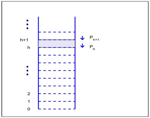
Figure for Exercise 1.11.7 Figure for Exercise 1.11.7.