1.7: Movement toward equilibrium

Now we consider a new mathematical model that is used to describe the response of systems to constant infusion of material or energy. Examples include

• A pristine lake has a constant flow of fresh water into it and an equal flow of water out of the lake. A factory is built next to the lake and each day releases a fixed amount of chemical waste into the lake. The chemical waste will mix through out the lake and some will leave the lake in the water flowing out. The amount of chemical waste in the lake will increase until the amount of chemical leaving the lake each day is the same as the amount released by the factory each day.
• The nitrogen in the muscle of a scuba diver is initially at 0.8 atm, the partial pressure of N₂ in atmospheric air. She descends to 20 meters and breathes air with N₂ partial pressure 2.4 atm. Almost immediately her blood N₂ partial pressure is also 2.4 atm. Her muscle absorbs N₂ more slowly; each minute the amount of N₂ that flows into her muscle is proportional to the difference between the partial pressures of N₂ in her blood (2.4 atm) and in her muscle. Gradually her muscle N₂ partial pressure moves toward 2.4 atm.
• A hen leaves a nest and exposes her eggs to air at temperatures that are lower than the \(37 ^{\circ} C\) of the eggs when she left. The temperature of the eggs will decrease toward the temperature of the air.

Example 1.7.1 Chemical pollution in a lake. A pristine lake of area 2 km² and average depth of 10 meters has a river flowing through it at a rate of 10,000 m³ per day. A factory is built beside the river and releases 100 kg of chemical waste into the lake each day. What will be the amounts of chemical waste in the lake on succeeding days? See Also: mathinsight.org/chemical_pollution_lake_model

We propose the following mathematical model.

Step 1. Mathematical Model. The daily change in chemical waste in the lake is difference between the amount released each day by the factory and the amount that flows out of the lake down the exit river. The amount of chemical waste that leaves the lake each day is equal to the amount of water that leaves the lake that day times the concentration of chemical waste in that water. Assume that upon release from the factory, the chemical quickly mixes throughout the lake so that the chemical concentration in the lake is uniform.

Step 2. Notation. Let \(t\) be time measured in days after the factory opens and \(W_t\) be the chemical waste in kg and \(C_t\) the concentration of chemical waste in \(kg/m^3\) in the lake on day \(t\). Let \(V\) be the volume of the lake and \(F\) the flow of water through the lake each day.

Step 3. Equations. The lake volume its area times its depth; according to the given data,

\[\begin{aligned}
&V=2 \mathrm{km}^{2} 10 \mathrm{m}=2 \cdot 10^{7} \mathrm{m}^{3}\\
&F=10^{4} \frac{\mathrm{m}^{3}}{\mathrm{day}}\\
&\text { The concentration of chemical in the lake is } \quad C_{t}=\frac{W_{t}}{V}=\frac{W_{t}}{2 \times 10^{7}} \frac{\mathrm{kg}}{\mathrm{m}^{3}}
\end{aligned}\]

The change in the amount of chemical on day \(t\) is \(W_{t+1} − W_{t}\) and

\[\begin{aligned}
\text{ Change per Day } &= \quad \text{ Amount Added per Day } &&− \quad \text{ Amount Removed per Day }\\
W_{t+1} - W_{t} &= \quad \quad \quad \quad \quad 100 &&- \quad \quad \quad \quad \quad F \cdot C_{t}\\
W_{t+1} - W_{t} &= \quad \quad \quad \quad \quad 100 \quad &&- \quad \quad \quad \quad \quad 10^{4} \frac{W_t}{2 \cdot 10^7}\\
W_{t+1} - W_{t} &= \quad \quad \quad \quad \quad 100 \quad &&- \quad \quad \quad \quad \quad 5 \cdot 10^{-4} W_{t}
\end{aligned}\]

The units in the equation are

\[\begin{aligned}
W_{t+1}-W_{t} &=100-10^{4} \frac{W_{t}}{2 \cdot 10^{7}} \\
\mathrm{kg}-\mathrm{kg} &=\mathrm{kg}-\mathrm{m}^{3} \frac{\mathrm{kg}}{\mathrm{m}^{3}}
\end{aligned}\]

and they are consistent.

On day 0, the chemical content of the lake is 0. Thus we have

\[\begin{aligned}
W_{0} &=0 \\
W_{t+1}-W_{t} &=100-5 \cdot 10^{-4} W_{t}
\end{aligned}\]

and we rewrite it as

\[\begin{aligned}
W_{0} &=0 \\
W_{t+1} &=100+0.9995 W_{t}
\end{aligned}\]

Step 5. Solve the dynamic equation. We can compute the amounts of chemical waste in the lake on the first few days¹³ and find 0, 100, 199.95, 299.85, 399.70 for the first five entries. We could iterate 365 times to find out what the chemical level will be at the end of one year (but would likely lose count).

Equilibrium State. The environmentalists want to know the ‘eventual state’ of the chemical waste in the lake. They would predict that the chemical in the lake will increase until there is no perceptual change on successive days. The equilibrium state is a number \(E\) such that if \(W_{t} = E, W_{t+1}\) is also \(E\). From \(W_{t+1} = 100 + 0.9995 W_{t}\) we write

\[E=100+0.9995 E, \quad E=\frac{100}{1-0.9995}=200,000\]

When the chemical in the lake reaches 200,000 kg, the amount that flows out of the lake each day will equal the amount introduced from the factory each day.

The equilibrium \(E\) is also useful mathematically. Subtract the equations

\[\begin{aligned}
W_{t+1} &=100+0.9995 W_{t} \\
E &=100+0.9995 E
\end{aligned}\]

\[W_{t+1}-E=0.9995\left(W_{t}-E\right)\]

With \(D_{t} = W_{t} − E\), this equation is

\[D_{t}+1=0.9995 D_{t} \quad \text{ which has the solution } \quad D_{t}=D_{0} 0.9995^{t}\]

Then

\[W_{t}-E=\left(W_{0}-E\right) 0.9995^{t}, \quad W_{t}=200000-200000 \cdot 0.9995^{t}\]

The graph of \(W_t\) is shown in Figure 1.7.1, and \(W_t\) is asymptotic to 200,000 kg.

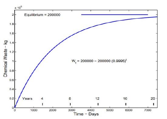
Figure \(\PageIndex{1}\): The amount of waste chemical in a lake.

You can read the chemical level of the lake at the end of one year from the graph or compute

\[W_{365}=200000-200000 \cdot 0.9995^{365} \doteq 33,000 kg\]

33,000 of the 36,500 kg of chemical released into the lake during the first year are still in the lake at the end of the year. Observe that even after 20 years the lake is not quite to equilibrium.

We can find out how long it takes for the lake to reach 98 percent of the equilibrium value by asking for what \(t\) is \(W_t = 0.98 \cdot 200000\)? Thus,

\[\begin{aligned}
W_{t}=0.98200000 &=200000-2000000.9995^{t} \\
0.98 &=1-0.9995^{t} \\
0.9995^{t} &=0.02 \\
\log 0.9995^{t} &=\log 0.02 \\
t \log 0.9995 &=\log 0.02 \\
t &=\frac{\log 0.02}{\log 0.9995}=7822 \quad \text { days }=21.4 \quad \text { years }
\end{aligned}\]

Step 6. Compare the solution with data. Unfortunately we do not have data for this model. The volume and stream flow were selected to approximate Lake Erie, but the lake is much more complex than our simple model. However, a simulation of the process is simple:

Example 1.7.2 Simulation of chemical discharge into a lake. Begin with two one-liter beakers, a supply of distilled water and salt and a meter to measure conductivity in water. Place one liter of distilled water and 0.5 g of salt in beaker F (factory). Place one liter of distilled water in beaker L (lake). Repeatedly do

1. Measure and record the conductivity of the water beaker L.
2. Remove 100 ml of solution from beaker L and discard.
3. Transfer 100 ml of salt water from beaker F to beaker L.

The conductivity of the salt water in beaker F should be about 1000 microsiemens (\(\mu S\)). The conductivity of the water in beaker L should be initially 0 and increase as the concentration of salt in L increases. Data and a graph of the data are shown in Figure 1.7.2 and appears similar to the graph in Figure 1.7.1. In Exercise 1.7.4 you are asked to write and solve a mathematical model of this simulation and and compare the solution with the data.

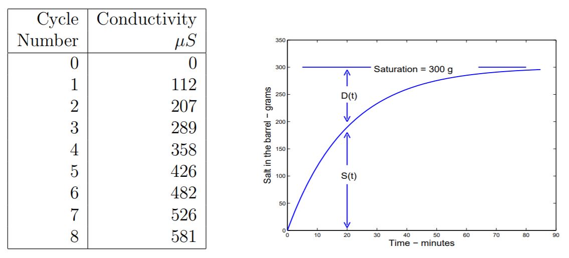
Figure \(\PageIndex{2}\): Data for Example 1.7.2, simulation of infusion of chemical waste product in a lake.

Exercises for Section 1.7 Movement toward equilibrium.

Exercise 1.7.1 For each of the following systems,

1. Compute \(W_{0}, W_{1}, W_{2}, W_{3}\), and \(W_4\).
2. Find the equilibrium value of Wt for the systems.
3. Write a solution equation for the system.
4. Compute \(W_{100}\).
5. Compute the half-life, \(T_{1/2} = − \frac{\log{2}}{\log{B}}\) of the system.
   1. \(\begin{aligned} W_{0} &= 0\\ W_{t+1} &= 1 - 0.2 W_{t} \end{aligned}\)
   2. \(\begin{aligned} W_{0} &= 0\\ W_{t+1} &= 10 - 0.2 W_{t} \end{aligned}\)
   3. \(\begin{aligned} W_{0} &= 0\\ W_{t+1} &= 100 - 0.2 W_{t} \end{aligned}\)
   4. \(\begin{aligned} W_{0} &= 0\\ W_{t+1} &= 10 - 0.1 W_{t} \end{aligned}\)
   5. \(\begin{aligned} W_{0} &= 0\\ W_{t+1} &= 10 - 0.05 W_{t} \end{aligned}\)
   6. \(\begin{aligned} W_{0} &= 0\\ W_{t+1} &= 10 - 0.01 W_{t} \end{aligned}\)

Exercise 1.7.3 For each of the following systems,

1. Compute \(W_{0}, W_{1}, W_{2}, W_{3}\), and \(W_{4}\).
2. Describe the future terms, \(W_{5}, W_{6}, W_{7}, \cdots\).
   1. \(\begin{aligned} W_{0} &= 0\\ W_{t+1} &= 1 - W_{t} \end{aligned}\)
   2. \(\begin{aligned} W_{0} &= \frac{1}{2}\\ W_{t+1} &= 1 - W_{t} \end{aligned}\)
   3. \(\begin{aligned} W_{0} &= 0\\ W_{t+1} &= 1 + W_{t} \end{aligned}\)
   4. \(\begin{aligned} W_{0} &= 0\\ W_{t+1} &= 2 + W_{t} \end{aligned}\)
   5. \(\begin{aligned} W_{0} &= 0\\ W_{t+1} &= 1 + 2 W_{t} \end{aligned}\)
   6. \(\begin{aligned} W_{0} &= -1\\ W_{t+1} &= 1 + 2 W_{t} \end{aligned}\)

Exercise 1.7.4 Write equations and solve them to describe the amount of salt in the beakers at the beginning of each cycle for the simulation of chemical discharge into a lake of Example 1.7.2.

Exercise 1.7.5 For our model, 1.7.1, of lake pollution, we assume “that upon release from the factory, the chemical quickly mixes throughout the lake so that the chemical concentration in the lake is uniform.” The time scale for ’quickly’ is relative to the other parts of the model; in this case to the daily flow into and out of the lake. Suppose it takes 10 days for 100 kg of chemical released from the factory to mix uniformly throughout the lake. Write a mathematical model for this case. There are several reasonable models; your task to write one of them.

Exercise 1.7.6 An intravenous infusion of penicillin is initiated into the vascular pool of a patient at the rate of 10 mg penicillin every five minutes. The patients kidneys remove 20 percent of the penicillin in the vascular pool every five minutes.

1. Write a mathematical model of the change during each five minute period of penicillin in the patient.
2. Write a difference equation that describes the amount of penicillin in the patient during the five minute intervals.
3. What is the initial value of penicillin in the patient?
4. What will be the equilibrium amount of penicillin in the patient? (This is important to the nurse and the doctor!)
5. Write a solution to the difference equation.
6. At what time will the penicillin amount in the patient reach 90 percent of the equilibrium value? (The nurse and doctor also care about this. Why?)
7. Suppose the patients kidneys are weak and only remove 10 percent of the penicillin in the vascular pool every 5 minutes. What is the equilibrium amount of penicillin in the patient?

Exercise 1.7.7 The nitrogen partial pressure in a muscle of a scuba diver is initially 0.8 atm. She descends to 30 meters and immediately the N₂ partial pressure in her blood is 2.4 atm, and remains at 2.4 atm while she remains at 30 meters. Each minute the N₂ partial pressure in her muscle increases by an amount that is proportional to the difference in 2.4 and the partial pressure of nitrogen in her muscle at the beginning of that minute.

1. Write a dynamic equation with initial condition to describe the N₂ partial pressure in her muscle.
2. Your dynamic equation should have a proportionality constant. Assume that constant to be 0.067. Write a solution to your dynamic equation.
3. At what time will the N₂ partial pressure be 1.6?
4. What is the half-life of N₂ partial pressure in the muscle, with the value of K = 0.067?

¹³ On your calculator: \(\begin{array}{cccccc}0 & \text { ENTER } & \times 0.9995+100 & \text { ENTER } & \text { ENTER } & \text { ENTER } & \text { ENTER }\end{array}\)