2.4: Polynomial Functions

Data from experiments (and their related functions) are often described as being linear, parabolic, hyperbolic, polynomial, harmonic (sines and cosines), exponential, or logarithmic either because their graphs have some resemblance to the corresponding geometric object or because equations describing their related functions use the corresponding expressions. In this section we extend linear and quadratic equations to more general polynomial functions.

Definition 2.3.1 Polynomial

For n a positive integer or zero, a polynomial of degree n is a function, P defined by an equation of the form

$$P(x)=a_{0}+a_{1} x+a_{2} x^{2}+a_{3} x^{3}+\cdots+a_{n} x^{n}$$

where $a_{0}, a_{1}, a_{2}, a_{3}, \cdots , a_{n}$ are numbers, independent of x, called the coefficients of p, and if $n > 0$ $a_{n} \neq 0$.

Functions of the form

$$P(x)=C \quad \text{where } C \text{ is a number}$$

are said to be constant functions and also polynomials of degree zero. Functions defined by equations

$$P(x)=a+b x \quad \text { and } \quad P(x)=a+b x+c x^{2}$$

are linear and quadratic polynomials, respectively, and are polynomials of degree one and degree two. The equation

$$P(x)=3+5 x+2 x^{2}+(-4) x^{3}$$

is a polynomial of degree 3 with coefficients 3, 5, 2, and -4 and is said to be a cubic polynomial.

Polynomials are important for four reasons:

1. Polynomials can be computed using only the arithmetic operations of addition, subtraction, and multiplication.
2. Most functions used in science have polynomials “close” to them over finite intervals. See Figure 2.4, Example 2.5.2, and Exercise 2.5.3.
3. The sum of two polynomials is a polynomial, the product of two polynomials is a polynomial, and the composition of two polynomials is a polynomial.
4. Polynomials are ‘linear’ in their coefficients, a fact which makes them suitable for least squares ‘fit’ to data.

Reason 1 is obvious, but even the meaning of Reason 2 is opaque. An illustration of Reason 2 follows, and we return to the question in Chapter 12. Sum, product, and composition of two functions are described in Section 2.6. Reason 4 is illustrated in Example 2.4.1.

A tangent to a graph is a polynomial of degree one ”close to” the graph. The graph of $F(x) = 2^x$ and the tangent

$$P_{1}(x)=1+0.69315 x \quad-1 \leq x \leq 2$$

at (0,1) are shown in Figure 2.4.1(a). The graph of the cubic polynomial

$$P_{3}(x)=1+0.69315 x+0.24023 x^{2}+0.05550 x^{3} \quad-1 \leq x \leq 2$$

shown in Figure 2.4.1(b) is even closer to the graph of $F(x) = 2^x$. These graphs are hardly distinguishable on $−1 \leq x \leq 1$ and only clearly separate at about $x = 1.5$. The function $F(x) = 2^x$ is difficult to evaluate (without a calculator) except at integer values of $x$, but $P_{3}(x)$ can be evaluated with just multiplication and addition. For $x = 0.5, F(0.5) = 2^{0.5} = \sqrt{2} = 1.41421$ and $P_{3}(0.5) = 1.41375$. The relative error in using $P_{3}(0.5)$ as an approximation to $\sqrt{2}$ is

$$\text { Relative Error } \quad=\left|\frac{P_{3}(0.5)-F(0.5)}{F(0.5)}\right|=\left|\frac{1.41375-1.41421}{1.41421}\right|=0.00033$$

The relative error is less than 0.04 percent.

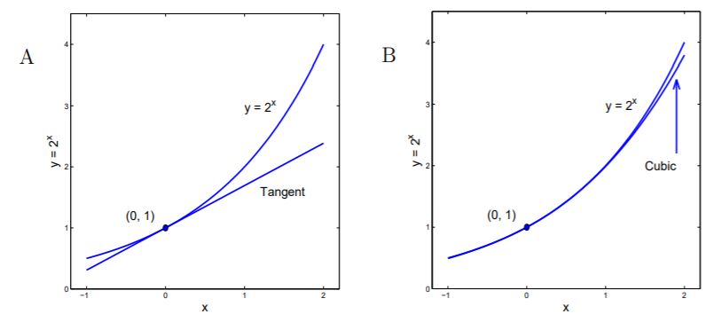
Figure $\PageIndex{1}$: A. Graph of $y = 2^x$ and its tangent at (0,1), $P_{1}(x) = 1 + 0.69315x$. B. Graph of $y = 2^x$ and the cubic, $P_{3}(x) = 1 + 0.69315 x + 0.24023 x^{2} + 0.05550 x^{3}$.

The tangent $P_{1}(x)$ is a good approximation to $F(x) = 2^x$ near the point of tangency (0,1) and the cubic polynomial $P_{3}(x)$ is an even better approximation. The coefficients 0.69135, 0.24023, and 0.05550 are presented here as Lightning Bolts Out of the Blue. A well defined procedure for selecting the coefficients is defined in Chapter 12.

Explore 2.4.1 Find the relative error in using the tangent approximation, $P_{1}(0.5) = 1 + 0.69315 \times 0.5$ as an approximation to $F(0.5) = 2^{0.5}$.

Example 2.4.1 Problem. Show that polynomials are linear in their coefficients. This means that

• The sum of two polynomials is obtained by adding ’corresponding’ coefficients (add the constant terms, add the coefficients of $x$, add the coefficients of $x^2$ , · · · ).
• The product of a constant, $K$, and a polynomial, $P(x)$, is the polynomial whose coefficients are the coefficients of $P(x)$ each multiplied by $K$.

Consider the following.

$$\begin{array}{l} \text { Let } P(x)=7-3 x+5 x^{2}, \quad \text { and } \quad Q(x)=-2+4 x-x^{2}+6 x^{3} \text { . } \\ \qquad \begin{aligned} P(x)+Q(x) &=\left(7-3 x+5 x^{2}\right)+\left(-2+4 x-x^{2}+6 x^{3}\right)\\ &=(7-2)+(-3+4) x+(5-1) x^{2}+(0+6) x^{3} \\ &=5+x+4 x^{2}+6 x^{3} \end{aligned} \end{array}$$

Thus $P(x) + Q(x)$ is simply the polynomial obtained by adding corresponding coefficients in $P(x)$ and $Q(x)$. Furthermore,

$$13 \cdot P(x)=13\left(7-3 x+5 x^{2}\right)=13 \cdot 7-13 \cdot 3 x+13 \cdot 5 x^{2}=91-39 x+65 x^{2}$$

Thus $13 \cdot P(x)$ is simply the polynomial obtained by multiplying each coefficient of $P(x)$ by 13. On the other hand, for

$$\begin{array}{c} P(x)=5 \sin 3 x, \quad Q(x)=6 \sin 4 x \\ P(x)+Q(x)=5 \sin 3 x+6 \sin 4 x \neq(5+6) \sin ((3+4) x)=11 \sin 7 x \end{array}$$

The sine functions are not linear in their coefficients.

 

Exercises for Section 2.4 Polynomial functions.

Exercise 2.4.1 Technology. Let \(F(x) = \sqrt{x}\). The polynomials

$$P_{2}(x)=\frac{3}{4}+\frac{3}{8} x-\frac{1}{64} x^{2} \quad \text { and } \quad P_{3}(x)=\frac{5}{8}+\frac{15}{32} x-\frac{5}{128} x^{2}+\frac{1}{512} x^{3}$$

closely approximate $F$ near the point (4,2) of $F$.

1. Draw the graphs of $F$ and $P_2$ on the range $1 \leq x \leq 8$.
2. Compute the relative error in $P_{2}(2)$ as an approximation to $F(2) = \sqrt{2}$.
3. Draw the graphs of $F$ and $P_{3}(x)$ on the range $1 \leq x \leq 8$.
4. Compute the relative error in $P_{3}(2)$ as an approximation to $F(2) = \sqrt{2}$.

Exercise 2.4.2 Technology. Let $F(x)=\sqrt[3]{x}$. The polynomials

$$P_{2}(x)=\frac{5}{9}+\frac{5}{9} x-\frac{1}{9} x^{2} \quad \text { and } \quad P_{3}(x)=P_{2}(x)+\frac{5}{81}(x-1)^{3}$$

closely approximate $F$ near the point (1,1) of $F$

1. Draw the graphs of $F$ and $P_2$ on the range $0 \leq x \leq 3$.
2. Compute the relative error in $P_{2}(2)$ as an approximation to \(F(2) = \sqrt[3]{2}).
3. Draw the graphs of $F$ and $P_3$ on the range $1 \leq x \leq 3$.
4. Compute the relative error in $P_{3}(2)$ as an approximation to $F(2) = \sqrt[3]{2}$.