
1.2: Solving Linear Equations
- Page ID
- 198266
\( \newcommand{\vecs}[1]{\overset { \scriptstyle \rightharpoonup} {\mathbf{#1}} } \)
\( \newcommand{\vecd}[1]{\overset{-\!-\!\rightharpoonup}{\vphantom{a}\smash {#1}}} \)
\( \newcommand{\dsum}{\displaystyle\sum\limits} \)
\( \newcommand{\dint}{\displaystyle\int\limits} \)
\( \newcommand{\dlim}{\displaystyle\lim\limits} \)
\( \newcommand{\id}{\mathrm{id}}\) \( \newcommand{\Span}{\mathrm{span}}\)
( \newcommand{\kernel}{\mathrm{null}\,}\) \( \newcommand{\range}{\mathrm{range}\,}\)
\( \newcommand{\RealPart}{\mathrm{Re}}\) \( \newcommand{\ImaginaryPart}{\mathrm{Im}}\)
\( \newcommand{\Argument}{\mathrm{Arg}}\) \( \newcommand{\norm}[1]{\| #1 \|}\)
\( \newcommand{\inner}[2]{\langle #1, #2 \rangle}\)
\( \newcommand{\Span}{\mathrm{span}}\)
\( \newcommand{\id}{\mathrm{id}}\)
\( \newcommand{\Span}{\mathrm{span}}\)
\( \newcommand{\kernel}{\mathrm{null}\,}\)
\( \newcommand{\range}{\mathrm{range}\,}\)
\( \newcommand{\RealPart}{\mathrm{Re}}\)
\( \newcommand{\ImaginaryPart}{\mathrm{Im}}\)
\( \newcommand{\Argument}{\mathrm{Arg}}\)
\( \newcommand{\norm}[1]{\| #1 \|}\)
\( \newcommand{\inner}[2]{\langle #1, #2 \rangle}\)
\( \newcommand{\Span}{\mathrm{span}}\) \( \newcommand{\AA}{\unicode[.8,0]{x212B}}\)
\( \newcommand{\vectorA}[1]{\vec{#1}} % arrow\)
\( \newcommand{\vectorAt}[1]{\vec{\text{#1}}} % arrow\)
\( \newcommand{\vectorB}[1]{\overset { \scriptstyle \rightharpoonup} {\mathbf{#1}} } \)
\( \newcommand{\vectorC}[1]{\textbf{#1}} \)
\( \newcommand{\vectorD}[1]{\overrightarrow{#1}} \)
\( \newcommand{\vectorDt}[1]{\overrightarrow{\text{#1}}} \)
\( \newcommand{\vectE}[1]{\overset{-\!-\!\rightharpoonup}{\vphantom{a}\smash{\mathbf {#1}}}} \)
\( \newcommand{\vecs}[1]{\overset { \scriptstyle \rightharpoonup} {\mathbf{#1}} } \)
\(\newcommand{\longvect}{\overrightarrow}\)
\( \newcommand{\vecd}[1]{\overset{-\!-\!\rightharpoonup}{\vphantom{a}\smash {#1}}} \)
\(\newcommand{\avec}{\mathbf a}\) \(\newcommand{\bvec}{\mathbf b}\) \(\newcommand{\cvec}{\mathbf c}\) \(\newcommand{\dvec}{\mathbf d}\) \(\newcommand{\dtil}{\widetilde{\mathbf d}}\) \(\newcommand{\evec}{\mathbf e}\) \(\newcommand{\fvec}{\mathbf f}\) \(\newcommand{\nvec}{\mathbf n}\) \(\newcommand{\pvec}{\mathbf p}\) \(\newcommand{\qvec}{\mathbf q}\) \(\newcommand{\svec}{\mathbf s}\) \(\newcommand{\tvec}{\mathbf t}\) \(\newcommand{\uvec}{\mathbf u}\) \(\newcommand{\vvec}{\mathbf v}\) \(\newcommand{\wvec}{\mathbf w}\) \(\newcommand{\xvec}{\mathbf x}\) \(\newcommand{\yvec}{\mathbf y}\) \(\newcommand{\zvec}{\mathbf z}\) \(\newcommand{\rvec}{\mathbf r}\) \(\newcommand{\mvec}{\mathbf m}\) \(\newcommand{\zerovec}{\mathbf 0}\) \(\newcommand{\onevec}{\mathbf 1}\) \(\newcommand{\real}{\mathbb R}\) \(\newcommand{\twovec}[2]{\left[\begin{array}{r}#1 \\ #2 \end{array}\right]}\) \(\newcommand{\ctwovec}[2]{\left[\begin{array}{c}#1 \\ #2 \end{array}\right]}\) \(\newcommand{\threevec}[3]{\left[\begin{array}{r}#1 \\ #2 \\ #3 \end{array}\right]}\) \(\newcommand{\cthreevec}[3]{\left[\begin{array}{c}#1 \\ #2 \\ #3 \end{array}\right]}\) \(\newcommand{\fourvec}[4]{\left[\begin{array}{r}#1 \\ #2 \\ #3 \\ #4 \end{array}\right]}\) \(\newcommand{\cfourvec}[4]{\left[\begin{array}{c}#1 \\ #2 \\ #3 \\ #4 \end{array}\right]}\) \(\newcommand{\fivevec}[5]{\left[\begin{array}{r}#1 \\ #2 \\ #3 \\ #4 \\ #5 \\ \end{array}\right]}\) \(\newcommand{\cfivevec}[5]{\left[\begin{array}{c}#1 \\ #2 \\ #3 \\ #4 \\ #5 \\ \end{array}\right]}\) \(\newcommand{\mattwo}[4]{\left[\begin{array}{rr}#1 \amp #2 \\ #3 \amp #4 \\ \end{array}\right]}\) \(\newcommand{\laspan}[1]{\text{Span}\{#1\}}\) \(\newcommand{\bcal}{\cal B}\) \(\newcommand{\ccal}{\cal C}\) \(\newcommand{\scal}{\cal S}\) \(\newcommand{\wcal}{\cal W}\) \(\newcommand{\ecal}{\cal E}\) \(\newcommand{\coords}[2]{\left\{#1\right\}_{#2}}\) \(\newcommand{\gray}[1]{\color{gray}{#1}}\) \(\newcommand{\lgray}[1]{\color{lightgray}{#1}}\) \(\newcommand{\rank}{\operatorname{rank}}\) \(\newcommand{\row}{\text{Row}}\) \(\newcommand{\col}{\text{Col}}\) \(\renewcommand{\row}{\text{Row}}\) \(\newcommand{\nul}{\text{Nul}}\) \(\newcommand{\var}{\text{Var}}\) \(\newcommand{\corr}{\text{corr}}\) \(\newcommand{\len}[1]{\left|#1\right|}\) \(\newcommand{\bbar}{\overline{\bvec}}\) \(\newcommand{\bhat}{\widehat{\bvec}}\) \(\newcommand{\bperp}{\bvec^\perp}\) \(\newcommand{\xhat}{\widehat{\xvec}}\) \(\newcommand{\vhat}{\widehat{\vvec}}\) \(\newcommand{\uhat}{\widehat{\uvec}}\) \(\newcommand{\what}{\widehat{\wvec}}\) \(\newcommand{\Sighat}{\widehat{\Sigma}}\) \(\newcommand{\lt}{<}\) \(\newcommand{\gt}{>}\) \(\newcommand{\amp}{&}\) \(\definecolor{fillinmathshade}{gray}{0.9}\)- Solving linear equations in one variable
- Interpret applications of linear equations
- Write linear equations in order to solve
- Classify linear equations
Linear equations are everywhere in the real world. When you try to figure how long it will take you to get home while driving a certain speed, or determining if you have enough money to pay your bills, you are solving a linear equation. In this section, we will practice solving some linear equations, create linear equations from given information, and examine applications of linear equations and slope intercept form. Usually, when a linear equation model uses real-world data, different letters are used for the variables, instead of using only x and y but you will still use the concept of slope and \(y\)-intercept (starting value or initial condition).
Solving Linear Equations in One Variable
A linear equation is an equation of a straight line, written in one variable. The only power of the variable is \(1\). Linear equations in one variable may take the form \(ax +b=0\) or \(ax +b=y\) where a number can be substituted in for \(y\), and are solved using basic algebraic operations. We begin by classifying linear equations in one variable as one of three types: identity, conditional, or inconsistent.
- An identity equation is true for all values of the variable. Here is an example of an identity equation: \[3x=2x+x \nonumber \] The solution set consists of all values that make the equation true. For this equation, the solution set is all real numbers because any real number substituted for \(x\) will make the equation true.
- A conditional equation is true for only some values of the variable. For example, if we are to solve the equation \(5x+2=3x−6\), we have the following: \[\begin{align*} 5x+2&=3x-6 \\ 2x &=-8 \\ x&=-4 \end{align*} \] The solution set consists of one number: \({−4}\). It is the only solution and, therefore, we have solved a conditional equation.
- An inconsistent equation results in a false statement. For example, if we are to solve \(5x−15=5(x−4)\), we have the following: \[\begin{align*} 5x−15 &=5x−20 \\ 5x−15-5x &= 5x−20-5x \\ −15 &\neq −20 \end{align*}\]Indeed, \(−15≠−20\). There is no solution because this is an inconsistent equation.
Solving linear equations in one variable involves the fundamental properties of equality and basic algebraic operations. A brief review of those operations follows.
Solve the following equation: \(2x+7=19\).
Solution
This equation can be written in the form \(ax +b=0\) by subtracting 19 from both sides. However, we may proceed to solve the equation in its original form by performing algebraic operations.
\[\begin{align*} 2x+7&=19\\ 2x&=12\qquad \text{Subtract 7 from both sides}\\ x&=6\qquad \text{Multiply both sides by } \dfrac{1}{2} \text{ or divide by } 2 \end{align*}\]
The solution is \(6\).
Solve the following equation: \(4(x−3)+12=15−5(x+6)\).
- Answer
-
Apply standard algebraic properties.
\[\begin{align*} 4(x-3)+12&=15-5(x+6)\\ 4x-12+12&=15-5x-30\qquad \text{Apply the distributive property by multipling by \(-5\) on the right }\\ 4x&=-15-5x\qquad \text{Combine like terms}\\ 9x&=-15\qquad \text{Place x terms on one side and simplify}\\ x&=-\dfrac{15}{9}\qquad \text{Multiply both sides by } \dfrac{1}{9} \text { , the reciprocal of } 9\\ x&=-\dfrac{5}{3} \end{align*}\]
Analysis
This problem requires the distributive property to be applied twice, and then the properties of algebra are used to reach the final line, \(x=-\dfrac{5}{3}\).
Solve a Formula for a Specific Variable
We have all probably worked with some geometric formulas in our study of mathematics. Formulas are used in so many fields, it is important to recognize formulas and be able to manipulate them easily.
It is often helpful to solve a formula for a specific variable. If you need to put a formula in a spreadsheet, it is not unusual to have to solve it for a specific variable first. We isolate that variable on one side of the equals sign with a coefficient of one and all other variables and constants are on the other side of the equal sign.
Geometric formulas often need to be solved for another variable, too. The formula \(V=\frac{1}{3}πr^2h\) is used to find the volume of a right circular cone when given the radius of the base and height. In the next example, we will solve this formula for the height.
Solve the formula \(V=\frac{1}{3}πr^2h\) for h.
- Answer
-
Write the formula. 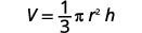
Remove the fraction on the right. 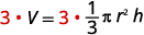
Simplify. 
Divide both sides by \(πr^2\). 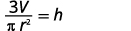
We could now use this formula to find the height of a right circular cone when we know the volume and the radius of the base, by using the formula \(h=\frac{3V}{πr^2}\).
1. Solve the formula \(C=\frac{5}{9}(F−32)\) for F. In the sciences we use Celsius as a measure of temperature.
- Answer
-
Write the formula. 
Remove the fraction on the right. 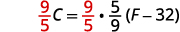
Simplify. 
Add 32 to both sides. 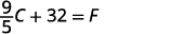
We can now use the formula \(F=\frac{9}{5}C+32\) to find the Fahrenheit temperature when we know the Celsius temperature.
Now solve your new equation for \(C\) and see if you can get back to the orginal equation.
2. Sometimes we solve for y so it is easier for us to graph. Solve the formula \(8x+7y=15\) for \(y\).
- Answer
-
Our goal is to isolate \(y\) on one side of the equation. 
Subtract \(6x\) from both sides to isolate the term with \(y\). 
Simplify. 
Divide both sides by \(7\) to make the coefficient of \(y\) one. 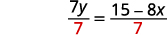
Simplify. 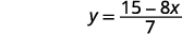
3. Solve the formula \(S=2πr^2+2πrh\) for \(h\). This is the formula for the surface area of a right cylinder.
- Answer
-
Write the formula. 
Isolate the \(h\) term by subtracting \(2πr^2\) from each side. 
Simplify. 
Solve for \(h\) by dividing both sides by \(2πr.\) 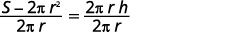
Simplify. 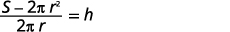
Using a Formula to Solve a Real-World Application
Many applications are solved using known formulas. The problem is stated, a formula is identified, the known quantities are substituted into the formula, the equation is solved for the unknown, and the problem’s question is answered. Typically, these problems involve two equations representing two trips, two investments, two areas, and so on. Examples of formulas include the area of a rectangular region,
\[A=LW \tag{2.4.2}\]
the perimeter of a rectangle,
\[P=2L+2W \tag{2.4.3}\]
and the volume of a rectangular solid,
\[V=LWH. \tag{2.4.4}\]
When there are two unknowns, we find a way to write one in terms of the other because we can solve for only one variable at a time.
It takes Andrew \(30\) minutes to drive to work in the morning. He drives home using the same route, but it takes \(10\) minutes longer, and he averages \(10\; mi/h\) less than in the morning. How far does Andrew drive to work?
Solution
This is a distance problem, so we can use the formula \(d =rt\), where distance equals rate multiplied by time. Note that when the rate is given in \(mi/h\), time must be expressed in hours. Consistent units of measurement are key to obtaining a correct solution.
First, we identify the known and unknown quantities. Andrew’s morning drive to work takes \(30\) minutes, or \(\frac{1}{2}\) hour at rate \(r\). His drive home takes \(40\) minutes or \(\frac{2}{3}\) of an hour, and his speed averages \(10\; mi/h\) less than the morning drive. Both trips cover distance \(d\). A table, such as Table \(\PageIndex{2}\), is often helpful for keeping track of information in these types of problems.
| \(d\) | \(r\) | \(t\) | |
|---|---|---|---|
| To Work | \(d\) | \(r\) | \(12\) |
| To Home | \(d\) | \(r−10\) | \(23\) |
Write two equations, one for each trip.
\[d=r\left(\dfrac{1}{2}\right) \qquad \text{To work} \nonumber\]
\[d=(r-10)\left(\dfrac{2}{3}\right) \qquad \text{To home} \nonumber\]
As both equations equal the same distance, we set them equal to each other and solve for \(r\).
\[\begin{align*} r\left (\dfrac{1}{2} \right )&= (r-10)\left (\dfrac{2}{3} \right )\\ \dfrac{1}{2}r&= \dfrac{2}{3}r-\dfrac{20}{3}\\ \dfrac{1}{2}r-\dfrac{2}{3}r&= -\dfrac{20}{3}\\ -\dfrac{1}{6}r&= -\dfrac{20}{3}\\ r&= -\dfrac{20}{3}(-6)\\ r&= 40 \end{align*}\]
We have solved for the rate of speed to work, \(40\; mph\). Substituting \(40\) into the rate on the return trip yields \(30\) mph Now we can answer the question. Substitute the rate back into either equation and solve for \(d\).
\[\begin{align*}d&= 40\left (\dfrac{1}{2} \right )\\ &= 20 \end{align*}\]
The distance between home and work is \(20\) miles..
Analysis
Note that we could have cleared the fractions in the equation by multiplying both sides of the equation by the LCD to solve for \(r\).
\[\begin{align*} r\left (\dfrac{1}{2} \right)&= (r-10)\left (\dfrac{2}{3} \right )\\ 6\times r\left (\dfrac{1}{2} \right)&= 6\times (r-10)\left (\dfrac{2}{3} \right )\\ 3r&= 4(r-10)\\ 3r&= 4r-40\\ r&= 40 \end{align*}\]
a. The perimeter of a rectangular outdoor patio is \(54\; ft\). The length is \(3\; ft\) greater than the width. What are the dimensions of the patio?
- Answer a
-
The perimeter formula is standard: \(P=2L+2W\). We have two unknown quantities, length and width. However, we can write the length in terms of the width as \(L =W+3\). Substitute the perimeter value and the expression for length into the formula. It is often helpful to make a sketch and label the sides as in Figure \(\PageIndex{3}\).
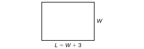
Figure \(\PageIndex{3}\) Now we can solve for the width and then calculate the length.
\[\begin{align*} P&= 2L + 2W\\ 54&= 2(W+3)+2W\\ 54&= 2W+6+2W\\ 54&= 4W+6\\ 48&= 4W\\ W&= 12 \end{align*}\]
\[\begin{align*} L&= 12+3\\ L&= 15 \end{align*}\]
The dimensions are \(L = 15\; ft\) and \(W = 12\; ft\).
b. The perimeter of a tablet of graph paper is \(48\space{in.}\). The length is \(6\; in\). more than the width. Find the area of the graph paper.
- Answer b
-
The standard formula for area is \(A =LW\); however, we will solve the problem using the perimeter formula. The reason we use the perimeter formula is because we know enough information about the perimeter that the formula will allow us to solve for one of the unknowns. As both perimeter and area use length and width as dimensions, they are often used together to solve a problem such as this one.
We know that the length is \(6\; in\). more than the width, so we can write length as \(L =W+6\). Substitute the value of the perimeter and the expression for length into the perimeter formula and find the length.
\[\begin{align*} P&= 2L + 2W\\ 48&= 2(W+6)+2W\\ 48&= 2W+12+2W\\ 48&= 4W+12\\ 36&= 4W\\ W&= 9 \end{align*}\]
\[\begin{align*}L&= 9+6\\ L&= 15 \end{align*}\]
Now, we find the area given the dimensions of \(L = 15\; in\). and \(W = 9\; in\).
\[\begin{align*} A&= LW\\ A&=15(9)\\ A&= 135\space{in.}^2 \end{align*}\]
The area is \(135\space{in.}^2\).
c. Find the dimensions of a shipping box given that the length is twice the width, the height is \(8\; \) in, and the volume is \(1,600\space{in.}^3\).
- Answer c
-
The formula for the volume of a box is given as \(V =LWH\), the product of length, width, and height. We are given that \(L =2W\), and \(H =8\). The volume is \(1,600\; \text{cubic inches}\).
\[\begin{align*} V&= LWH\\ 1600&= (2W)W(8)\\ 1600&= 16W^2\\ 100&= W^2\\ 10&= W \end{align*}\]The dimensions are \(L = 20\; in\), \(W= 10\; in\), and \(H = 8\; in\).
Analysis
Note that the square root of \(W^2\) would result in a positive and a negative value. However, because we are describing width, we can use only the positive result.
d. Find a linear equation to solve for the following unknown quantities: One number exceeds another number by \( 17\) and their sum is \( 31\). Find the two numbers.
- Answer d
-
Let \( x\) equal the first number. Then, as the second number exceeds the first by \(17\), we can write the second number as \( x +17\). The sum of the two numbers is \(31\). We usually interpret the word is as an equal sign.
\[\begin{align*} x+(x+17)&= 31\\ 2x+17&= 31\\ 2x&= 14\\ x&= 7 \end{align*}\]
\[\begin{align*} x+17&= 7 + 17\\ &= 24\\ \end{align*}\]
The two numbers are \(7\) and \(24\).
Classify Equations
Whether or not an equation is true depends on the value of the variable. The equation \(7x+8=−13\) is true when we replace the variable, x, with the value \(−3\), but not true when we replace x with any other value. An equation like this is called a conditional equation. All the equations we have solved so far are conditional equations.
Now let’s consider the equation \(7y+14=7(y+2)\). Do you recognize that the left side and the right side are equivalent? Let’s see what happens when we solve for y.
Solve:
| \(7 y+14=7(y+2)\) | |
| Distribute. | \(7 y+14=7 y+14\) |
| Subtract \(7y\) to each side to get the \(y’\)s to one side. | \(7 y \color{red}-7 y \color{black} +14=7 y \color{red} -7 y \color{black}+14\) |
| Simplify—the \(y\)'s are eliminated. | \(14=14\) |
| But \(14=14\) is true. |
This means that the equation \(7y+14=7(y+2)\) is true for any value of \(y\). We say the solution to the equation is all of the real numbers. An equation that is true for any value of the variable is called an identity.
What happens when we solve the equation \(−8z=−8z+9?\)
Solve:
| \(-8 z=-8 z+9\) | |
| Add \(8z\) to both sides to leave the constant alone on the right. | \(-8 z \color{red} +8 z \color{black}=-8 z \color{red}+8 z \color{black} +9\) |
| Simplify—the \(z\)'s are eliminated. | \(0 \neq 9\) |
| But \(0≠9\). |
Solving the equation \(−8z=−8z+9\) led to the false statement \(0=9\). The equation \(−8z=−8z+9\) will not be true for any value of \(z\). It has no solution. An equation that has no solution, or that is false for all values of the variable, is called a contradiction.
We summarize the methods for classifying equations in the table.
| Type of Equation | What happens when you solve it? | Solution |
|---|---|---|
| Conditional Equation | True for one or more values of the variables and false for all other values | One or more values |
| Identity | True for any value of the variable | All real numbers |
| Contradiction | False for all values of the variable | No solution |
Solve Equations with Fraction or Decimal Coefficients
We could use the General Strategy to solve the next example. This method would work fine, but many students do not feel very confident when they see all those fractions. So, we are going to show an alternate method to solve equations with fractions. This alternate method eliminates the fractions.
We will apply the Multiplication Property of Equality and multiply both sides of an equation by the least common denominator (LCD) of all the fractions in the equation. The result of this operation will be a new equation, equivalent to the first, but without fractions. This process is called clearing the equation of fractions.
To clear an equation of decimals, we think of all the decimals in their fraction form and then find the LCD of those denominators.
Solve: \(\frac{1}{12}x+\frac{5}{6}=\frac{3}{4}\).
- Answer
-

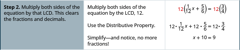
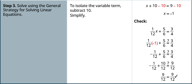
Notice in the previous example, once we cleared the equation of fractions, the equation was like those we solved earlier in this chapter. We changed the problem to one we already knew how to solve. We then used the General Strategy for Solving Linear Equations.
Solve: \(5=\frac{1}{2}y+\frac{2}{3}y−\frac{3}{4}y\).
- Answer
-
We want to clear the fractions by multiplying both sides of the equation by the LCD of all the fractions in the equation.
Find the LCD of all fractions in the equation. \(5=\frac{1}{2} y+\frac{2}{3} y-\frac{3}{4} y\) The LCD is \(12\). Multiply both sides of the equation by \(12\). \(\color{red}12 \color{black}(5)=\color{red}12 \color{black} \cdot\left(\frac{1}{2} y+\frac{2}{3} y-\frac{3}{4} y\right)\) Distribute. \(12(5)=12 \cdot \frac{1}{2} y+12 \cdot \frac{2}{3} y-12 \cdot \frac{3}{4} y\) Simplify—notice, no more fractions. \(60=6 y+8 y-9 y\) Combine like terms. \(60=5 y\) Divide by five. \(\frac{60}{\color{red}5} \color{black}=\frac{5 y}{\color{red}5}\) Simplify. \(12=y\) Check: \(5=\frac{1}{2} y+\frac{2}{3} y-\frac{3}{4} y\) Let \(y=12\). 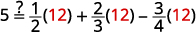

a. Solve: \(\frac{1}{2}(y−5)=\frac{1}{4}(y−1)\).
- Answer
-
In this example, we will distribute before we clear the fractions. Do not stress if you did it differently.

Distribute. 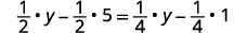
Simplify. 
Multiply by the LCD, four. 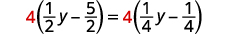
Distribute. 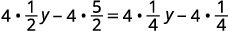
Simplify. 
Collect the variables to the left. 
Simplify. 
Collect the constants to the right. 
Simplify. 
An alternate way to solve this equation is to clear the fractions without distributing first. If you multiply the factors correctly, this method will be easier. 
Multiply by the LCD, \(4\). 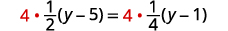
Multiply four times the fractions. 
Distribute. 
Collect the variables to the left. .jpg?revision=1&size=bestfit&width=228&height=17)
Simplify. 
Collect the constants to the right. 
Simplify. 
Check: 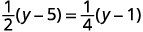
Let \(y=9\). 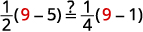
b. Solve: \(0.25x+0.05(x+3)=2.85\).
- Answer
-

Distribute first. 
Combine like terms. 
To clear decimals, multiply by \(100\). 
Distribute. 
Subtract \(15\) from both sides. 
Simplify. 
Divide by \(30\). 
Simplify. 
Some equations have decimals in them. This kind of equation may occur when we solve problems dealing with money or percentages. But decimals can also be expressed as fractions. For example, \(0.7=\frac{7}{10}\) and \(0.29=\frac{29}{100}\). So, with an equation with decimals, we can use the same method we used to clear fractions—multiply both sides of the equation by the least common denominator.
Key Concepts
- A linear equation can be used to solve for an unknown in a number problem.
- Applications can be written as mathematical problems by identifying known quantities and assigning a variable to unknown quantities.
- Classify equations as conditional, identity, or contradiction.
- Solve linear equations with decimals and fractions.
- Classify equations as conditional, identity, or contradiction.