
1.1: Finding Distances and Midpoints
- Page ID
- 193546

\( \newcommand{\vecs}[1]{\overset { \scriptstyle \rightharpoonup} {\mathbf{#1}} } \)
\( \newcommand{\vecd}[1]{\overset{-\!-\!\rightharpoonup}{\vphantom{a}\smash {#1}}} \)
\( \newcommand{\dsum}{\displaystyle\sum\limits} \)
\( \newcommand{\dint}{\displaystyle\int\limits} \)
\( \newcommand{\dlim}{\displaystyle\lim\limits} \)
\( \newcommand{\id}{\mathrm{id}}\) \( \newcommand{\Span}{\mathrm{span}}\)
( \newcommand{\kernel}{\mathrm{null}\,}\) \( \newcommand{\range}{\mathrm{range}\,}\)
\( \newcommand{\RealPart}{\mathrm{Re}}\) \( \newcommand{\ImaginaryPart}{\mathrm{Im}}\)
\( \newcommand{\Argument}{\mathrm{Arg}}\) \( \newcommand{\norm}[1]{\| #1 \|}\)
\( \newcommand{\inner}[2]{\langle #1, #2 \rangle}\)
\( \newcommand{\Span}{\mathrm{span}}\)
\( \newcommand{\id}{\mathrm{id}}\)
\( \newcommand{\Span}{\mathrm{span}}\)
\( \newcommand{\kernel}{\mathrm{null}\,}\)
\( \newcommand{\range}{\mathrm{range}\,}\)
\( \newcommand{\RealPart}{\mathrm{Re}}\)
\( \newcommand{\ImaginaryPart}{\mathrm{Im}}\)
\( \newcommand{\Argument}{\mathrm{Arg}}\)
\( \newcommand{\norm}[1]{\| #1 \|}\)
\( \newcommand{\inner}[2]{\langle #1, #2 \rangle}\)
\( \newcommand{\Span}{\mathrm{span}}\) \( \newcommand{\AA}{\unicode[.8,0]{x212B}}\)
\( \newcommand{\vectorA}[1]{\vec{#1}} % arrow\)
\( \newcommand{\vectorAt}[1]{\vec{\text{#1}}} % arrow\)
\( \newcommand{\vectorB}[1]{\overset { \scriptstyle \rightharpoonup} {\mathbf{#1}} } \)
\( \newcommand{\vectorC}[1]{\textbf{#1}} \)
\( \newcommand{\vectorD}[1]{\overrightarrow{#1}} \)
\( \newcommand{\vectorDt}[1]{\overrightarrow{\text{#1}}} \)
\( \newcommand{\vectE}[1]{\overset{-\!-\!\rightharpoonup}{\vphantom{a}\smash{\mathbf {#1}}}} \)
\( \newcommand{\vecs}[1]{\overset { \scriptstyle \rightharpoonup} {\mathbf{#1}} } \)
\(\newcommand{\longvect}{\overrightarrow}\)
\( \newcommand{\vecd}[1]{\overset{-\!-\!\rightharpoonup}{\vphantom{a}\smash {#1}}} \)
\(\newcommand{\avec}{\mathbf a}\) \(\newcommand{\bvec}{\mathbf b}\) \(\newcommand{\cvec}{\mathbf c}\) \(\newcommand{\dvec}{\mathbf d}\) \(\newcommand{\dtil}{\widetilde{\mathbf d}}\) \(\newcommand{\evec}{\mathbf e}\) \(\newcommand{\fvec}{\mathbf f}\) \(\newcommand{\nvec}{\mathbf n}\) \(\newcommand{\pvec}{\mathbf p}\) \(\newcommand{\qvec}{\mathbf q}\) \(\newcommand{\svec}{\mathbf s}\) \(\newcommand{\tvec}{\mathbf t}\) \(\newcommand{\uvec}{\mathbf u}\) \(\newcommand{\vvec}{\mathbf v}\) \(\newcommand{\wvec}{\mathbf w}\) \(\newcommand{\xvec}{\mathbf x}\) \(\newcommand{\yvec}{\mathbf y}\) \(\newcommand{\zvec}{\mathbf z}\) \(\newcommand{\rvec}{\mathbf r}\) \(\newcommand{\mvec}{\mathbf m}\) \(\newcommand{\zerovec}{\mathbf 0}\) \(\newcommand{\onevec}{\mathbf 1}\) \(\newcommand{\real}{\mathbb R}\) \(\newcommand{\twovec}[2]{\left[\begin{array}{r}#1 \\ #2 \end{array}\right]}\) \(\newcommand{\ctwovec}[2]{\left[\begin{array}{c}#1 \\ #2 \end{array}\right]}\) \(\newcommand{\threevec}[3]{\left[\begin{array}{r}#1 \\ #2 \\ #3 \end{array}\right]}\) \(\newcommand{\cthreevec}[3]{\left[\begin{array}{c}#1 \\ #2 \\ #3 \end{array}\right]}\) \(\newcommand{\fourvec}[4]{\left[\begin{array}{r}#1 \\ #2 \\ #3 \\ #4 \end{array}\right]}\) \(\newcommand{\cfourvec}[4]{\left[\begin{array}{c}#1 \\ #2 \\ #3 \\ #4 \end{array}\right]}\) \(\newcommand{\fivevec}[5]{\left[\begin{array}{r}#1 \\ #2 \\ #3 \\ #4 \\ #5 \\ \end{array}\right]}\) \(\newcommand{\cfivevec}[5]{\left[\begin{array}{c}#1 \\ #2 \\ #3 \\ #4 \\ #5 \\ \end{array}\right]}\) \(\newcommand{\mattwo}[4]{\left[\begin{array}{rr}#1 \amp #2 \\ #3 \amp #4 \\ \end{array}\right]}\) \(\newcommand{\laspan}[1]{\text{Span}\{#1\}}\) \(\newcommand{\bcal}{\cal B}\) \(\newcommand{\ccal}{\cal C}\) \(\newcommand{\scal}{\cal S}\) \(\newcommand{\wcal}{\cal W}\) \(\newcommand{\ecal}{\cal E}\) \(\newcommand{\coords}[2]{\left\{#1\right\}_{#2}}\) \(\newcommand{\gray}[1]{\color{gray}{#1}}\) \(\newcommand{\lgray}[1]{\color{lightgray}{#1}}\) \(\newcommand{\rank}{\operatorname{rank}}\) \(\newcommand{\row}{\text{Row}}\) \(\newcommand{\col}{\text{Col}}\) \(\renewcommand{\row}{\text{Row}}\) \(\newcommand{\nul}{\text{Nul}}\) \(\newcommand{\var}{\text{Var}}\) \(\newcommand{\corr}{\text{corr}}\) \(\newcommand{\len}[1]{\left|#1\right|}\) \(\newcommand{\bbar}{\overline{\bvec}}\) \(\newcommand{\bhat}{\widehat{\bvec}}\) \(\newcommand{\bperp}{\bvec^\perp}\) \(\newcommand{\xhat}{\widehat{\xvec}}\) \(\newcommand{\vhat}{\widehat{\vvec}}\) \(\newcommand{\uhat}{\widehat{\uvec}}\) \(\newcommand{\what}{\widehat{\wvec}}\) \(\newcommand{\Sighat}{\widehat{\Sigma}}\) \(\newcommand{\lt}{<}\) \(\newcommand{\gt}{>}\) \(\newcommand{\amp}{&}\) \(\definecolor{fillinmathshade}{gray}{0.9}\)- Find the distance between two points
- Find the midpoint between two points
- Apply the distance and midpoint formulas
Using the Distance Formula
Derived from the Pythagorean Theorem, the distance formula is used to find the distance between two points in the plane. The Pythagorean Theorem, \(a^2+b^2=c^2\), is based on a right triangle where \(a\) and \(b\) are the lengths of the legs adjacent to the right angle, and \(c\) is the length of the hypotenuse. See Figure \(\PageIndex{1}\).
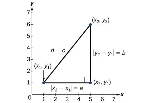
The relationship of sides \(|x_2−x_1|\) and \(|y_2−y_1|\) to side \(d\) is the same as that of sides \(a\) and \(b\) to side \(c\). We use the absolute value symbol to indicate that the length is a positive number because the absolute value of any number is positive. (For example, \(|-3|=3\). ) The symbols \(|x_2−x_1|\) and \(|y_2−y_1|\) indicate that the lengths of the sides of the triangle are positive. To find the length \(c\), take the square root of both sides of the Pythagorean Theorem.
\[c^2=a^2+b^2\rightarrow c=\sqrt{a^2+b^2}\]
It follows that the distance formula is given as
\[d^2={(x_2−x_1)}^2+{(y_2−y_1)}^2\rightarrow d=\sqrt{{(x_2−x_1)}^2+{(y_2−y_1)}^2}\]
We do not have to use the absolute value symbols in this definition because any number squared is positive.
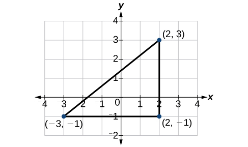
Find the distance between the points \((−3,−1)\) and \((2,3)\).
Solution
Let us first look at the graph of the two points. Connect the points to form a right triangle as in Figure \(\PageIndex{2}\)
Then, calculate the length of \(d\) using the distance formula.
One option would be to count along the horizontal leg of the triangle. The number of boxes from \(-3\) to \(2\) is \(5\) which is also the distance traveled. Notice these numbers are the \(x\)-coordinates of two ordered pairs. Now count the number of boxes along the vertical leg of the triangle from \(-1\) to \( 3\), resulting in a distance traveled of \(4\). Notice these are the \(y\)-coordinates of the two points.
We may not wish to draw the triangle on fancy graph paper, but we have a formula to use instead. Notice the process and results are the same.
\[\begin{align*} d&= \sqrt{{(x_2 - x_1)}^2+{(y_2 - y_1)}^2}\\ &= \sqrt{{(2-(-3))}^2+{(3-(-1))}^2}\\ &= \sqrt{{(5)}^2+{(4)}^2}\\ &= \sqrt{25+16}\\ &= \sqrt{41} \end{align*}\]
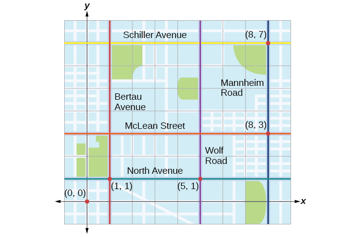
Tracie set out from Elmhurst, IL \((0,0)\), to go to Franklin Park \((8.7)\). On the way, she made a few stops to do errands. Each stop is indicated by a red dot at \((1,1)\), \((5,1)\),and \((8,3)\).(. Find the total distance that Tracie traveled. Compare this with the distance between her starting and final positions.

Solution
The first thing we should do is identify ordered pairs to describe each position. If we set the starting position at the origin, we can identify each of the other points by counting units east (right) and north (up) on the grid. For example, the first stop is \(1\) block east and \(1\) block north, so it is at \((1,1)\). The next stop is \(5\) blocks to the east, so it is at \((5,1)\). After that, she traveled \(3\) blocks east and \(2\) blocks north to \((8,3)\). Lastly, she traveled \(4\) blocks north to \((8,7)\). We can label these points on the grid as in Figure \(\PageIndex{3}\).
Next, we can calculate the distance. Note that each grid unit represents \(1,000\) feet.
- From her starting location to her first stop at \((1,1)\), Tracie might have driven north \(1,000\) feet and then east \(1,000\) feet, or vice versa. Either way, she drove \(2,000\) feet to her first stop.
- Her second stop is at \((5,1)\). So from \((1,1)\) to \((5,1)\), Tracie drove east \(4,000\) feet.
- Her third stop is at \((8,3)\). There are a number of routes from \((5,1)\) to \((8,3)\). Whatever route Tracie decided to use, the distance is the same, as there are no angular streets between the two points. Let’s say she drove east \(3,000\) feet and then north \(2,000\) feet for a total of \(5,000\) feet.
- Tracie’s final stop is at \((8,7)\). This is a straight drive north from \((8,3)\) for a total of \(4,000\) feet.
Next, we will add the distances listed in Table \(\PageIndex{4}\).
| From/To | Number of Feet Driven |
|---|---|
| \((0,0)\) to \((1,1)\) | \(2,000\) |
| \((1,1)\) to \((5,1)\) | \(4,000\) |
| \((5,1)\) to \((8,3)\) | \(5,000\) |
| \((8,3)\) to \((8,7)\) | \(4,000\) |
| Total | \(15,000\) |
The total distance Tracie drove is \(15,000\) feet, or \(2.84\) miles.
- Find the distance between two points: \((1,4)\) and \((11,9)\).
- Answer a
- If we choose not to use a graph, we can use our formula and see that \[\begin{align*} d&= \sqrt{{(11-1)}^2+{(9-4)}^2}\\ &= \sqrt{100+25}\\ &= \sqrt{125}\\ &= 5\sqrt{5}\ \approx 11.18 \end{align*}\]
b. In Example 2, we found that Traci drove \(15,000\) feet, however this is not the actual distance between her starting and ending positions. Find the distance, "as the crow flies" between her starting and ending positions.
- Answer b
-
To find this distance, we can use the distance formula between the points \((0,0)\) and \((8,7)\).
\[\begin{align*} d&= \sqrt{{(0-8)}^2+{(7-0)}^2}\\ &= \sqrt{64+49}\\ &= \sqrt{113}\ \approx 10.63 \text{ units} \end{align*}\]
At \(1,000\) feet per grid unit, the distance between Elmhurst, IL, to Franklin Park is \(10,630.14\) feet, or \(2.01\) miles. The distance formula results in a shorter calculation because it is based on the hypotenuse of a right triangle, a straight diagonal from the origin to the point \((8,7)\). Perhaps you have heard the saying “as the crow flies,” which means the shortest distance between two points because a crow can fly in a straight line, even though a person on the ground has to travel a longer distance on existing roadways.
Using the Midpoint Formula
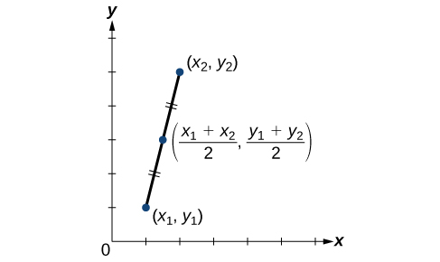
When the endpoints of a line segment are known, we can find the point midway between them. This point is known as the midpoint (or the average between the two points), and the formula is known as the midpoint formula. Given the endpoints of a line segment, \((x_1,y_1)\) and \((x_2,y_2)\), the midpoint formula allows us to find the average of the x- and y-coordinates to determine the coordinates of the midpoint M.
\[M=\left (\dfrac{x_1+x_2}{2}, \dfrac{y_1+y_2}{2} \right )\]
A graphical view of a midpoint is shown in Figure \(\PageIndex{5}\). Notice that the line segments on either side of the midpoint are congruent.
Find the midpoint of the line segment with the endpoints \((7,−2)\) and \((9,5)\).
Solution
Use the formula to find the midpoint of the line segment.
\[\begin{align*} \left (\dfrac{x_1+x_2}{2},\dfrac{y_1+y_2}{2} \right )&= \left (\dfrac{7+9}{2},\dfrac{-2+5}{2} \right )\\ &= \left (8,\dfrac{3}{2} \right ) \end{align*}\]
- Find the midpoint of the line segment with endpoints \((−2,−1)\) and \((−8,6)\).
- The diameter of a circle has endpoints \((−1,−4)\) and \((5,−4)\). Find the center of the circle.
- Answer a
- \(\left (-5,\dfrac{5}{2} \right )\)
- Answer b
-
The center of a circle is the center, or midpoint, of its diameter. Thus, the midpoint formula will yield the center point.
\[\begin{align*} \left (\dfrac{x_1+x_2}{2},\dfrac{y_1+y_2}{2} \right )&= \left (\dfrac{-1+5}{2},\dfrac{-4-4}{2}) \right )\\ &= \left (\dfrac{4}{2},-\dfrac{8}{2} \right )\\ &= (2,4) \end{align*}\]
Key Concepts
- The distance formula is derived from the Pythagorean Theorem and is used to find the length of a line segment.
- The midpoint formula provides a method of finding the coordinates of the midpoint dividing the sum of the \(x\)-coordinates and the sum of the \(y\)-coordinates of the endpoints by \(2\).