3.6: Zeros of Polynomial Functions

Learning Objectives

• Evaluate a polynomial using the Remainder Theorem.
• Use the Factor Theorem to solve a polynomial equation.
• Find zeros of a polynomial function.
• Use the Linear Factorization Theorem to find polynomials with given zeros.
• Solve real-world applications of polynomial equations

A new bakery offers decorated sheet cakes for children’s birthday parties and other special occasions. The bakery wants the volume of a small cake to be 351 cubic inches. The cake is in the shape of a rectangular solid. They want the length of the cake to be four inches longer than the width of the cake and the height of the cake to be one-third of the width. What should the dimensions of the cake pan be?

This problem can be solved by writing a cubic function and solving a cubic equation for the volume of the cake. In this section, we will discuss a variety of tools for writing polynomial functions and solving polynomial equations.

Evaluating a Polynomial Using the Remainder Theorem

In the last section, we learned how to divide polynomials. We can now use polynomial division to evaluate polynomials using the Remainder Theorem. If the polynomial is divided by \(x–k\), the remainder may be found quickly by evaluating the polynomial function at \(k\), that is, \(f(k)\). Let’s walk through the proof of the theorem.

Recall that the Division Algorithm states that, given a polynomial dividend \(f(x)\) and a non-zero polynomial divisor \(d(x)\) where the degree of \(d(x)\) is less than or equal to the degree of \(f(x)\), there exist unique polynomials \(q(x)\) and \(r(x)\) such that

\[f(x)=d(x)q(x)+r(x) \nonumber\]

If the divisor, \(d(x)\), is \(x−k\), this takes the form

\[f(x)=(x−k)q(x)+r \nonumber\]

Since the divisor \(x−k\)

is linear, the remainder will be a constant, \(r\). And, if we evaluate this for \(x=k\), we have

\[\begin{align*} f(k)&=(k−k)q(k)+r \\[4pt] &=0{\cdot}q(k)+r \\[4pt] &=r \end{align*}\]

In other words, \(f(k)\) is the remainder obtained by dividing \(f(x)\)by \(x−k\).

Example \(\PageIndex{1}\): Using the Remainder Theorem to Evaluate a Polynomial

Use the Remainder Theorem to evaluate \(f(x)=6x^4−x^3−15x^2+2x−7\) at \(x=2\).

Solution

To find the remainder using the Remainder Theorem, use synthetic division to divide the polynomial by \(x−2\).

\[ 2 \begin{array}{|ccccc} \; 6 & −1 & −15 & 2 & −7 \\ \text{} & 12 & 22 & 14 & 32 \\ \hline \end{array} \\ \begin{array}{ccccc} 6 & 11 & \; 7 & \;\;16 & \;\; 25 \end{array} \]

The remainder is 25. Therefore, \(f(2)=25\).

Analysis

We can check our answer by evaluating \(f(2)\).

\[\begin{align*} f(x)&=6x^4−x^3−15x^2+2x−7 \\ f(2)&=6(2)^4−(2)^3−15(2)^2+2(2)−7 \\ &=25 \end{align*}\]

Using the Factor Theorem to Solve a Polynomial Equation

The Factor Theorem is another theorem that helps us analyze polynomial equations. It tells us how the zeros of a polynomial are related to the factors. Recall the Division Algorithm.

\[f(x)=(x−k)q(x)+r\]

If \(k\) is a zero, then the remainder \(r\) is \(f(k)=0\) and \(f (x)=(x−k)q(x)+0\) or \(f(x)=(x−k)q(x)\).

Notice, written in this form, \(x−k\) is a factor of \(f(x)\). We can conclude if \(k\) is a zero of \(f(x)\), then \(x−k\) is a factor of \(f(x)\).

Similarly, if \(x−k\) is a factor of \(f(x)\), then the remainder of the Division Algorithm \(f(x)=(x−k)q(x)+r\) is \(0\). This tells us that \(k\) is a zero.

This pair of implications is the Factor Theorem. As we will soon see, a polynomial of degree \(n\) in the complex number system will have \(n\) zeros. We can use the Factor Theorem to completely factor a polynomial into the product of \(n\) factors. Once the polynomial has been completely factored, we can easily determine the zeros of the polynomial.

Example \(\PageIndex{2}\): Using the Factor Theorem to Solve a Polynomial Equation

Show that \((x+2)\) is a factor of \(x^3−6x^2−x+30\). Find the remaining factors. Use the factors to determine the zeros of the polynomial.

Solution

We can use synthetic division to show that \((x+2)\) is a factor of the polynomial.

\[ -2 \begin{array}{|cccc} \; 1 & −6 & −1 & 30 \\ \text{} & -2 & 16 & -30 \\ \hline \end{array} \\ \begin{array}{cccc} 1 & -8 & \; 15 & \;\;0 \end{array} \]

The remainder is zero, so \((x+2)\) is a factor of the polynomial. We can use the Division Algorithm to write the polynomial as the product of the divisor and the quotient:

\[(x+2)(x^2−8x+15)\]

We can factor the quadratic factor to write the polynomial as

\[(x+2)(x−3)(x−5)\]

By the Factor Theorem, the zeros of \(x^3−6x^2−x+30\) are –2, 3, and 5.

Finding the Zeros of Polynomial Functions

Technology can help us narrow down the list of possible rational zeros for a polynomial function. Once we have an integer solution, we can use synthetic division repeatedly to determine all of the zeros of a polynomial function.

Example \(\PageIndex{3}\):  Finding Zeros of a Polynomial

List all zeros of \(f(x)=2x^{3}+x^{2}-4x+1\).

Solution

Since \(f(x)\) is of degree \(3\), there must be three solutions. Use technology to determine if there are any integer or rational zeros.  

 

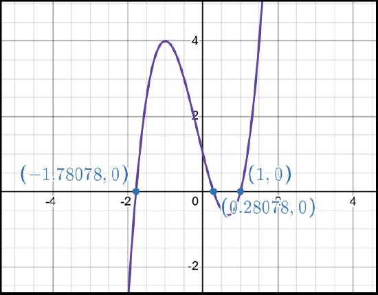
Graphically, we can see that \(x=1\) is a solution.  From previous sections we know that \(f(1))=0\) and that \((x-1)\) is a factor of the polynomial.  

Use synthetic division to find the other solutions.  Using the coefficients \(2, 1, -4, 1\) and the divisor of \(1\) we get

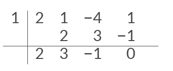
Dividing a cubic by a linear term, results in the quotient of \(2x^2+3x-1\), which is a quadratic.  Now choose to solve the quadratic equation through factoring or the quadratic formula.  Recognizing that it does not factor, use the quadratic formula.  

Identify the coefficients: \(a=2,b=3,c=-1\). Then use the quadratic formula.

\[\begin{align*} x&= \dfrac{-3 \pm \sqrt{(3)^2-4(2)(-1)}}{2(2)}\\ &= \dfrac{-3 \pm \sqrt{9+8}}{4}\\ &= \dfrac{-5 \pm \sqrt{17}}{4} \end{align*}\]

The zeros of the polynomial are \(x=1, x=\dfrac{-5 + \sqrt{17}}{4}, x=\dfrac{-5 - \sqrt{17}}{4}\)

The zeros of the polynomial are \(x=1, x\thickapprox 0.28078, x\thickapprox -1.78078\) which can be verified graphically.

Exercise \(\PageIndex{1}\)

Find the zeros of \(f(x)=x^{4}+4x^{3}-4x^{2}-32x-32\).

Answer

Since \(f(x)\) is of degree \(4\), there must be four solutions. Use technology to determine if there are any integer or rational zeros.  

 

Graphically, we can see that \(x=-2\) is a solution.  From previous sections we know that \(f(-2))=0\) and that \((x+2)\) is a factor of the polynomial. Since the graph bounces off at \(x=-2\), \(-2\) is a zero of multiplicity \(2\).

Use synthetic division to find the other solutions.  Using the coefficients \(1, 4, -4, -32, -32\) and the divisor of \(2\) we get

Dividing a fourth degree by a linear term results in the cubic of \(x^3+2x^2-8x-16\).  Noticing that \(-2\) is a double root, divide again by \(-2\).

Dividing a cubic by a linear term results in the quadratic of \(x^2-8\). 

First, set the equation equal to zero: \(x^2-8=0\).

Then add \(8\) to both sides:  \(x^2=8\).

Take the square root of both sides, and then simplify the radical. Remember to use a \(±\) sign before the radical symbol.

\[\begin{align*} x^2&= 8\\ x&= \pm \sqrt{8}\\ &= \pm 2\sqrt{2} \end{align*}\]

The solutions to the quadratic are \(2\sqrt{2}\),\(-2\sqrt{2}\)

The zeros of the polynomial are \(x=2, x=2, x=2\sqrt(2), x=-2\sqrt(2)

The zeros of the polynomial are \(x=2 (\text{multiplicity} 2), x\thickapprox -2.82843, x\thickapprox -2.82843\) which can be verified graphically.

You may be asking yourself, Why do I need to go through all of these steps and divide when I can just get the approximations from Desmos. This is a very good question.  Unfortunately, I do not have an answer to this question.  We want you to be able to think.  Just believing what the computer tells you is not a good plan for your life.  Additionally, just think how much fun you are having.

Using the Fundamental Theorem of Algebra

Now that we can find rational zeros for a polynomial function, we will look at a theorem that discusses the number of complex zeros of a polynomial function. The Fundamental Theorem of Algebra tells us that every polynomial function has at least one complex zero. This does not mean that every polynomial has at least one imaginary solution as can be seen in previous examples. Real numbers are a subset of the complex numbers but not the other way around. This theorem forms the foundation for solving polynomial equations.

Suppose \(f\) is a polynomial function of degree four, and \(f (x)=0\). The Fundamental Theorem of Algebra states that there is at least one complex solution, call it \(c_1\). By the Factor Theorem, we can write \(f(x)\) as a product of \(x−c_1\) and a polynomial quotient. Since \(x−c_1\) is linear, the polynomial quotient will be of degree three. Now we apply the Fundamental Theorem of Algebra to the third-degree polynomial quotient. It will have at least one complex zero, call it \(c_2\). So we can write the polynomial quotient as a product of \(x−c_2\) and a new polynomial quotient of degree two. Continue to apply the Fundamental Theorem of Algebra until all of the zeros are found. There will be four of them and each one will yield a factor of \(f(x)\).

Example \(\PageIndex{4}\): Finding the Zeros of a Polynomial Function with Complex Zeros

Find the zeros of \(f(x)=3x^3+9x^2+x+3\).

Solution

Since \(f(x)\) is of degree \(3\), there must be three solutions. Use technology to determine if there are any integer or rational zeros.  

 

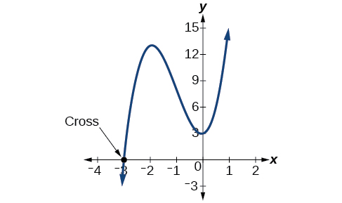
Graphically, we can see that \(x=-3\) is a solution.  From previous sections we know that \(f(-3))=0\) and that \((x+3)\) is a factor of the polynomial. Notice that the graph of the polynomial does not cross the x-axis anywhere else. This is your clue that all other solutions must be imaginary solutions. The process to find these solutions is the same as before. 

Use synthetic division to find the other solutions.  Using the coefficients \(3, 9, 1, 3\) and the divisor of \(-3\) we get

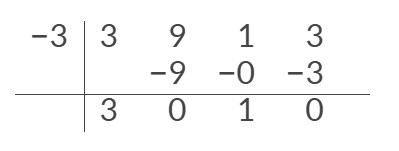
Dividing a cubic by a linear term, results in the quotient of \(3x^2+1\), which is a quadratic.  The polynomial can now be written as \[(x+3)(3x^2+1) \nonumber\]

We can then set the quadratic equal to 0 and solve to find the other zeros of the function.

First, set the equation equal to zero: \(3x^2+1=0\).

Then subtract \(1\) from both sides:  \(3x^2=-1\).

Divide both sides by \(3\):  \(x^2=\frac{-1}{3}\).

Take the square root of both sides, and then simplify the radical. Remember to use a \(±\) sign before the radical symbol.

\[\begin{align*} x^2&= \frac{-1}{3} \\ x&= \pm \sqrt{\dfrac{-1}{3}}\\ &= \pm i\dfrac{\sqrt{3}}{3} \end{align*}\]

The solutions to the quadratic are \(\dfrac{i\sqrt{3}}{3}\),\(-\dfrac{i\sqrt{3}}{3}\)

The roots of the polynomial are \(x=-3, x=\dfrac{i\sqrt{3}}{3}, x=-\dfrac{i\sqrt{3}}{3}\) 

Since the roots are imaginary, we cannot verify graphically.  

Analysis

Look at the graph of the function \(f\) in Figure \(\PageIndex{2}\). Notice that, at \(x =−3\), the graph crosses the x-axis, indicating an odd multiplicity (1) for the zero \(x=–3\). Also note the presence of the two turning points. This means that, since there is a \(3^{rd}\) degree polynomial, we are looking at the maximum number of turning points. So, the end behavior of increasing without bound to the right and decreasing without bound to the left will continue. Thus, all the x-intercepts for the function are shown. So either the multiplicity of \(x=−3\) is 1 and there are two complex solutions, which is what we found, or the multiplicity at \(x =−3\) is three. Either way, our result is correct.

Figure \(\PageIndex{1}\).

Using the Linear Factorization Theorem to Find Polynomials with Given Zeros

A vital implication of the Fundamental Theorem of Algebra, as we stated above, is that a polynomial function of degree n will have \(n\) zeros in the set of complex numbers, if we allow for multiplicities. This means that we can factor the polynomial function into \(n\) factors. The Linear Factorization Theorem tells us that a polynomial function will have the same number of factors as its degree, and that each factor will be in the form \((x−c)\), where c is a complex number.

Let \(f\) be a polynomial function with real coefficients, and suppose \(a +bi\), \(b≠0\), is a zero of \(f(x)\). Then, by the Factor Theorem, \(x−(a+bi)\) is a factor of \(f(x)\). For \(f\) to have real coefficients, \(x−(a−bi)\) must also be a factor of \(f(x)\). This is true because any factor other than \(x−(a−bi)\), when multiplied by \(x−(a+bi)\), will leave imaginary components in the product. Only multiplication with conjugate pairs will eliminate the imaginary parts and result in real coefficients. In other words, if a polynomial function \(f\) with real coefficients has a complex zero \(a +bi\), then the complex conjugate \(a−bi\) must also be a zero of \(f(x)\). This is called the Complex Conjugate Theorem.

Example \(\PageIndex{5}\): Using the Linear Factorization Theorem to Find a Polynomial with Given Zeros

Find a fourth degree polynomial with real coefficients that has zeros of \(–3\), \(2\), \(i\), such that \(f(−2)=100\).

Solution

Because \(x =i\) is a zero, by the Complex Conjugate Theorem \(x =–i\) is also a zero. The polynomial must have factors of \((x+3),(x−2),(x−i)\), and \((x+i)\). Since we are looking for a degree 4 polynomial, and now have four zeros, we have all four factors. Let’s begin by multiplying these factors.

\[\begin{align} f(x) & =a(x+3)(x−2)(x−i)(x+i) \\ f(x) & =a(x^2+x−6)(x^2+1) \\ f(x) & =a(x^4+x^3−5x^2+x−6) \end{align} \]

We need to find \(a\) to ensure \(f(–2)=100\). Substitute \(x=–2\) and \(f (-2)=100\) into \(f (x)\).

\[\begin{align} 100=a({(−2)}^4+{(−2)}^3−5{(−2)}^2+(−2)−6) \\ 100=a(−20) \\ −5=a \end{align} \]

So the polynomial function is

\[f(x)=−5(x^4+x^3−5x^2+x−6)\]

or

\[f(x)=−5x^4−5x^3+25x^2−5x+30\] Analysis

We found that both \(i\) and \(−i\) were zeros, but only one of these zeros needed to be given. If \(i\) is a zero of a polynomial with real coefficients, then \(−i\) must also be a zero of the polynomial because \(−i\) is the complex conjugate of \(i\).

Solving Real-World Applications

We have now introduced a variety of tools for solving polynomial equations. Let’s use these tools to solve the bakery problem from the beginning of the section.

Example \(\PageIndex{6}\)

A new bakery offers decorated sheet cakes for children’s birthday parties and other special occasions. The bakery wants the volume of a small cake to be 351 cubic inches. The cake is in the shape of a rectangular solid. They want the length of the cake to be four inches longer than the width of the cake and the height of the cake to be one-third of the width. What should the dimensions of the cake pan be?

Solution

Begin by writing an equation for the volume of the cake. The volume of a rectangular solid is given by \(V=lwh\). We were given that the length must be four inches longer than the width, so we can express the length of the cake as \(l=w+4\). We were given that the height of the cake is one-third of the width, so we can express the height of the cake as \(h=\dfrac{1}{3}w\). Let’s write the volume of the cake in terms of width of the cake.

\[V=(w+4)(w)(\dfrac{1}{3}w)\] \[V=\dfrac{1}{3}w^3+\dfrac{4}{3}w^2\]

Substitute the given volume into this equation.

\(351=13w^3+43w^2\) Substitute 351 for V. \(1053=w^3+4w^2\) Multiply both sides by 3. \(0=w^3+7w^2−1053\) Subtract 1053 from both sides.

Descartes' rule of signs tells us there is one positive solution. The Rational Zero Theorem tells us that the possible rational zeros are \(\pm 1,±3,±9,±13,±27,±39,±81,±117,±351,\) and \(±1053\). We can use synthetic division to test these possible zeros. Only positive numbers make sense as dimensions for a cake, so we need not test any negative values. Let’s begin by testing values that make the most sense as dimensions for a small sheet cake. Use synthetic division to check \(x=1\).

Since 1 is not a solution, we will check \(x=3\).

Since 3 is not a solution either, we will test \(x=9\).

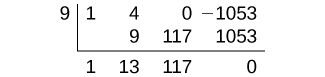
Synthetic division gives a remainder of 0, so 9 is a solution to the equation. We can use the relationships between the width and the other dimensions to determine the length and height of the sheet cake pan.

\(l=w+4=9+4=13\) and \(h=\dfrac{1}{3}w=\dfrac{1}{3}(9)=3\)

The sheet cake pan should have dimensions 13 inches by 9 inches by 3 inches

 

Key Concepts

• To find \(f(k)\), determine the remainder of the polynomial \(f(x)\) when it is divided by \(x−k\). This is known as the Remainder Theorem. 
• According to the Factor Theorem, \(k\) is a zero of \(f(x)\) if and only if \((x−k)\) is a factor of \(f(x)\). 
• When the leading coefficient is 1, the possible rational zeros are the factors of the constant term.
• Synthetic division can be used to find the zeros of a polynomial function. 
• According to the Fundamental Theorem, every polynomial function with degree greater than 0 has at least one complex zero. 
• Allowing for multiplicities, a polynomial function will have the same number of factors as its degree. Each factor will be in the form \((x−c)\), where \(c\) is a complex number.