
3.7: Polynomial Inequalities
- Page ID
- 206095

\( \newcommand{\vecs}[1]{\overset { \scriptstyle \rightharpoonup} {\mathbf{#1}} } \)
\( \newcommand{\vecd}[1]{\overset{-\!-\!\rightharpoonup}{\vphantom{a}\smash {#1}}} \)
\( \newcommand{\dsum}{\displaystyle\sum\limits} \)
\( \newcommand{\dint}{\displaystyle\int\limits} \)
\( \newcommand{\dlim}{\displaystyle\lim\limits} \)
\( \newcommand{\id}{\mathrm{id}}\) \( \newcommand{\Span}{\mathrm{span}}\)
( \newcommand{\kernel}{\mathrm{null}\,}\) \( \newcommand{\range}{\mathrm{range}\,}\)
\( \newcommand{\RealPart}{\mathrm{Re}}\) \( \newcommand{\ImaginaryPart}{\mathrm{Im}}\)
\( \newcommand{\Argument}{\mathrm{Arg}}\) \( \newcommand{\norm}[1]{\| #1 \|}\)
\( \newcommand{\inner}[2]{\langle #1, #2 \rangle}\)
\( \newcommand{\Span}{\mathrm{span}}\)
\( \newcommand{\id}{\mathrm{id}}\)
\( \newcommand{\Span}{\mathrm{span}}\)
\( \newcommand{\kernel}{\mathrm{null}\,}\)
\( \newcommand{\range}{\mathrm{range}\,}\)
\( \newcommand{\RealPart}{\mathrm{Re}}\)
\( \newcommand{\ImaginaryPart}{\mathrm{Im}}\)
\( \newcommand{\Argument}{\mathrm{Arg}}\)
\( \newcommand{\norm}[1]{\| #1 \|}\)
\( \newcommand{\inner}[2]{\langle #1, #2 \rangle}\)
\( \newcommand{\Span}{\mathrm{span}}\) \( \newcommand{\AA}{\unicode[.8,0]{x212B}}\)
\( \newcommand{\vectorA}[1]{\vec{#1}} % arrow\)
\( \newcommand{\vectorAt}[1]{\vec{\text{#1}}} % arrow\)
\( \newcommand{\vectorB}[1]{\overset { \scriptstyle \rightharpoonup} {\mathbf{#1}} } \)
\( \newcommand{\vectorC}[1]{\textbf{#1}} \)
\( \newcommand{\vectorD}[1]{\overrightarrow{#1}} \)
\( \newcommand{\vectorDt}[1]{\overrightarrow{\text{#1}}} \)
\( \newcommand{\vectE}[1]{\overset{-\!-\!\rightharpoonup}{\vphantom{a}\smash{\mathbf {#1}}}} \)
\( \newcommand{\vecs}[1]{\overset { \scriptstyle \rightharpoonup} {\mathbf{#1}} } \)
\(\newcommand{\longvect}{\overrightarrow}\)
\( \newcommand{\vecd}[1]{\overset{-\!-\!\rightharpoonup}{\vphantom{a}\smash {#1}}} \)
\(\newcommand{\avec}{\mathbf a}\) \(\newcommand{\bvec}{\mathbf b}\) \(\newcommand{\cvec}{\mathbf c}\) \(\newcommand{\dvec}{\mathbf d}\) \(\newcommand{\dtil}{\widetilde{\mathbf d}}\) \(\newcommand{\evec}{\mathbf e}\) \(\newcommand{\fvec}{\mathbf f}\) \(\newcommand{\nvec}{\mathbf n}\) \(\newcommand{\pvec}{\mathbf p}\) \(\newcommand{\qvec}{\mathbf q}\) \(\newcommand{\svec}{\mathbf s}\) \(\newcommand{\tvec}{\mathbf t}\) \(\newcommand{\uvec}{\mathbf u}\) \(\newcommand{\vvec}{\mathbf v}\) \(\newcommand{\wvec}{\mathbf w}\) \(\newcommand{\xvec}{\mathbf x}\) \(\newcommand{\yvec}{\mathbf y}\) \(\newcommand{\zvec}{\mathbf z}\) \(\newcommand{\rvec}{\mathbf r}\) \(\newcommand{\mvec}{\mathbf m}\) \(\newcommand{\zerovec}{\mathbf 0}\) \(\newcommand{\onevec}{\mathbf 1}\) \(\newcommand{\real}{\mathbb R}\) \(\newcommand{\twovec}[2]{\left[\begin{array}{r}#1 \\ #2 \end{array}\right]}\) \(\newcommand{\ctwovec}[2]{\left[\begin{array}{c}#1 \\ #2 \end{array}\right]}\) \(\newcommand{\threevec}[3]{\left[\begin{array}{r}#1 \\ #2 \\ #3 \end{array}\right]}\) \(\newcommand{\cthreevec}[3]{\left[\begin{array}{c}#1 \\ #2 \\ #3 \end{array}\right]}\) \(\newcommand{\fourvec}[4]{\left[\begin{array}{r}#1 \\ #2 \\ #3 \\ #4 \end{array}\right]}\) \(\newcommand{\cfourvec}[4]{\left[\begin{array}{c}#1 \\ #2 \\ #3 \\ #4 \end{array}\right]}\) \(\newcommand{\fivevec}[5]{\left[\begin{array}{r}#1 \\ #2 \\ #3 \\ #4 \\ #5 \\ \end{array}\right]}\) \(\newcommand{\cfivevec}[5]{\left[\begin{array}{c}#1 \\ #2 \\ #3 \\ #4 \\ #5 \\ \end{array}\right]}\) \(\newcommand{\mattwo}[4]{\left[\begin{array}{rr}#1 \amp #2 \\ #3 \amp #4 \\ \end{array}\right]}\) \(\newcommand{\laspan}[1]{\text{Span}\{#1\}}\) \(\newcommand{\bcal}{\cal B}\) \(\newcommand{\ccal}{\cal C}\) \(\newcommand{\scal}{\cal S}\) \(\newcommand{\wcal}{\cal W}\) \(\newcommand{\ecal}{\cal E}\) \(\newcommand{\coords}[2]{\left\{#1\right\}_{#2}}\) \(\newcommand{\gray}[1]{\color{gray}{#1}}\) \(\newcommand{\lgray}[1]{\color{lightgray}{#1}}\) \(\newcommand{\rank}{\operatorname{rank}}\) \(\newcommand{\row}{\text{Row}}\) \(\newcommand{\col}{\text{Col}}\) \(\renewcommand{\row}{\text{Row}}\) \(\newcommand{\nul}{\text{Nul}}\) \(\newcommand{\var}{\text{Var}}\) \(\newcommand{\corr}{\text{corr}}\) \(\newcommand{\len}[1]{\left|#1\right|}\) \(\newcommand{\bbar}{\overline{\bvec}}\) \(\newcommand{\bhat}{\widehat{\bvec}}\) \(\newcommand{\bperp}{\bvec^\perp}\) \(\newcommand{\xhat}{\widehat{\xvec}}\) \(\newcommand{\vhat}{\widehat{\vvec}}\) \(\newcommand{\uhat}{\widehat{\uvec}}\) \(\newcommand{\what}{\widehat{\wvec}}\) \(\newcommand{\Sighat}{\widehat{\Sigma}}\) \(\newcommand{\lt}{<}\) \(\newcommand{\gt}{>}\) \(\newcommand{\amp}{&}\) \(\definecolor{fillinmathshade}{gray}{0.9}\)- Solve polynomial inequalities
We have solved polynomial equations; now we will solve polynomial inequalities. We will ue some of the techniques learned when solving linear and quadratic functions. We will also solve polynomial inequalities both graphically and algebraically.
Recall that multiplying or dividing by a negative number on both sides of an inequality changes the direction of the inequality sign.
\[\begin{array}{cccc}
& -2 x \leq-6 & \Longrightarrow & x {\color{Red} \geq } 3 \\
\text { but } & 2 x \leq 6 & \Longrightarrow & x \leq 3
\end{array} \nonumber \]
Solve Polynomial Inequalities Algebraically & Graphically
A polynomial equation is in standard form when written as \(a_0x^n+a_1x^{n-1} + . . . a_{n-1}x+a_n=0\). If we replace the equal sign with an inequality, we have a polynomial inequality in standard form. In previous sections, we studied the end behavior of polynomials of odd and even degrees, as well as several methods for determining x-intercepts. Recall from our work with quadratics, when we ask if \(a_0x^n+a_1x^{n-1} + . . . a_{n-1}x+a_n>0\) we want to know when the function is greater than \(0\) i.e. above the x-axis.
We will use a three-step strategy to solve these inequalities. First, we solve the polynomial using factoring, graphing, and division. The second step is to look at subintervals based on the solutions. Finally, we check the endpoints of each interval.
- Solve: \(x^2-3x-4\geq 0\)
Algebraic Solution
We can find the roots of the polynomial by factoring \(x^2-3x-4= 0\).
\((x-4)(x+1)=0\) implies the solution is \(x=4\) or \(x=-1\)
Then we can use a number line and check solutions in each interval.
By plotting the two points on the x-axis we see that there are three separate regions to consider: \((-\infty,-1)\), \((-1,4)\), and \((4,\infty)\)
Choosing a random x-value in each region will allow us to check if the answer is positive (above the x-axis) or negative (below the x-axis).
In the figure below, we choose \(-3\) in the first region, \(0\) in the second region [authors note: always choose zero if it is an option], and \(5\) in the last region.
For example, \(f(-3)=14\). However, any number chosen in the interval \((-\infty,-1)\) would result in a positive answer. We see that \(f(0)=-4\), however, any number in the interval \((-1,4)\) would result in a negative number. Finally, \(f(5)=6\), but again, any number chosen from the interval \((4,\infty)\) would result in a positive number.

Therefore, the answer to our question \(x^2-3x-4\geq 0\) is \[\{x|x\leq -1,\text{ or }x\geq 4\}=(-\infty,-1]\cup [4,\infty) \nonumber \]
Graphical Solution
To see where \(f(x)=x^2-3x-4\) is \(\geq 0\), we graph it with Desmos.

We see that \(f(x)\geq 0\) when \(x\leq -1\) and when \(x\geq 4\) (the parts of the graph above the \(x\)-axis). The solution set is therefore
\[\{x|x\leq -1,\text{ or }x\geq 4\}=(-\infty,-1]\cup [4,\infty) \nonumber \]
Solve: \(x^3-9x^2+23x-15\leq 0\)
Algebraic Solution
We can find the roots of the polynomial using our previously learned skills concerning solving polynomials.
Notice that \(f(1) = (1)^3-9(1)^2+23(1)-15\leq 0\) which implies that \(1\) is a solution.
Using synthetic division, we find the quadratic term.

Now, factoring \(x^2-8x+15=(x-5)(x-3)=0\) leads to the other solutions of \(x=5\) or \(x=3\)
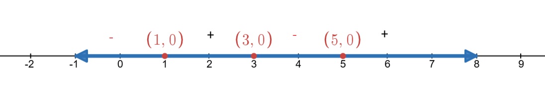
Then we can use a number line and check solutions in each interval.
By plotting the two points on the x-axis we see that there are four separate regions to consider: \((-\infty,1)\), \((1,3\), ((3,5\), and \((5,\infty)\)
Choosing a random x-value in each region will allow us to determine if the function values in each region are positive (above the x-axis) or negative (below the x-axis).
In the figure below, we choose \(x=0\) resulting in \(-15\) in the first region, \(x=2\) in the second region, \(x=4\) in the third region, and \(x=10\) in the last region.
However, any number chosen in the interval \((-\infty,1)\) would result in a negative answer. We see that \(f(2)=3\), however, any number in the interval \((1,3)\) would result in a positive number. While \(f(4)=-3\), any number in the interval \((3,5)\) would result in a negative number. Finally, \(f(10)=315\), but again, any number chosen from the interval \((5,\infty)\) would result in a positive number.
\[\begin{aligned} \text{solution set}&=\{x\in \mathbb{R} | x\leq 1, \text{ or } 3\leq x\leq 5\} \\ &=(-\infty,1]\cup [3,5] \end{aligned} \nonumber \]
Note that we include the roots \(1\), \(3\), and \(5\) in the solution set since the original inequality was “\(\leq\)” (and not “\(<\)”), which includes the solutions of the corresponding equality.
Graphical Solution
Here is the graph of the function \(f(x)=x^3-9x^2+23x-15\)

This graph shows that there are two intervals where \(f(x)\leq 0\) (the parts of the graph below the \(x\)-axis). To determine the exact intervals, we calculate where \(f(x)=x^3-9x^2+23x-15=0\). The graph suggests that the roots of \(f(x)\) are at \(x=1\), \(x=3\), and \(x=5\). This can be confirmed by a calculation:
\[\begin{aligned} f(1)&= 1^3-9\cdot 1^2+23\cdot 1-15=1-9+23-15=0\\ f(3)&= 3^3-9\cdot 3^2+23\cdot 3-15=27-81+69-15=0\\ f(5)&= 5^3-9\cdot 5^2+23\cdot 5-15=125-225+115-15=0\end{aligned} \nonumber \]
Since \(f\) is a polynomial of degree \(3\), the roots \(x=1, 3, 5\) are all of the roots of \(f\). (Alternatively, we could have divided \(f(x)\), for example, by \(x-1\) and used this to completely factor \(f\) and with this obtain all the roots of \(f\).) With this, we can determine the solution set to be the set:
\[\begin{aligned} \text{solution set}&=\{x\in \mathbb{R} | x\leq 1, \text{ or } 3\leq x\leq 5\} \\ &=(-\infty,1]\cup [3,5] \end{aligned} \nonumber \]
Note that we include the roots \(1\), \(3\), and \(5\) in the solution set since the original inequality was “\(\leq\)” (and not “\(<\)”), which includes the solutions of the corresponding equality.
Solve: \(x^4-x^2 > 5(x^3-x)\)
Algebraic Solution
To factor and easily interpret the solutions, we rewrite the inequality to obtain zero on one side.
\[\begin{aligned}
x^{4}-x^{2}>5\left(x^{3}-x\right) (\text { distribute } 5) & \Longrightarrow \quad x^{4}-x^{2}>5 x^{3}-5 x \\
\left(\text { subtract } 5 x^{3}, \text{ add } 5 x\right) & \Longrightarrow \quad x^{4}-5 x^{3}-x^{2}+5 x>0
\end{aligned} \nonumber \]
We can find the roots of the polynomial using our previously learned skills concerning solving polynomials.
Notice that there is a common term in each pair of terms.
\(x^3(x-5) - x(x-5)=0\)
\((x^3-x)(x-5)=0\)
Giving two equations to solve \(x^3-x=0 and x-5=0\)
Which implies that \(-1\) \(0\) \(1\) and \(5\) are solutions.
Then we can use a number line and check solutions in each interval.
By plotting the four points on the x-axis and choosing a random point in each interval, we see there are three regions that give positive solutions and two regions that give a negative solutions.

\[\begin{aligned} \text{solution set}&=\{x\in \mathbb{R} | x\leq 1, \text{ or } 3\leq x\leq 5\} \\ &=(-\infty,1]\cup [3,5] \end{aligned} \nonumber \]
Note that we include the roots \(1\), \(3\), and \(5\) in the solution set since the original inequality was “\(\leq\)” (and not “\(<\)”), which includes the solutions of the corresponding equality.
Graphical Solution
In order to graph and easily interpret the solutions, we rewrite the inequality to obtain zero on one side of the inequality.
\[\begin{aligned}
x^{4}-x^{2}>5\left(x^{3}-x\right) (\text { distribute } 5) & \Longrightarrow \quad x^{4}-x^{2}>5 x^{3}-5 x \\
\left(\text { subtract } 5 x^{3}, \text{ add } 5 x\right) & \Longrightarrow \quad x^{4}-5 x^{3}-x^{2}+5 x>0
\end{aligned} \nonumber \]
We graph \(f(x)=x^4-5x^3-x^2+5x\).

The graph suggests the roots \(x=-1\), \(0\), \(1\), and \(5\) which can be confirmed by a straightforward calculation.
\[\begin{aligned} f(-1)&= (-1)^4-5\cdot (-1)^3-(-1)^2+5\cdot (-1)=1+5-1-5=0\\ f(0)&= 0^4-5\cdot 0^3-0^2-5\cdot 0=0\\ f(1)&= 1^4-5\cdot 1^3-1^2+5\cdot 1=1-5-1+5=0\\ f(5)&= 5^4-5\cdot 5^3-5^2+5\cdot 5=125-125-25+25=0\end{aligned} \nonumber \]
The roots \(x=-1\), \(0\), \(1\), and \(5\) are the only roots since \(f\) is of degree \(4\). The intervals of the solution for \(f(x)>0\) may be read off from the graph:
\[\text{solution set}=(-\infty,-1)\cup (0,1)\cup (5, \infty) \nonumber \]
(Notice that the roots \(-1\), \(0\), \(1\), and \(5\) are not included in the solution set since our inequality reads \(f(x)>0\) and not \(f(x)\geq 0\).)
Solve: \(x^3+15x>7x^2+9\)
- Answer
-
First, bring all terms to one side. It does not matter whether we bring the terms to the right or the left side of the inequality sign! The resulting inequality is different, but the solution to the problem is the same.
\[x^3+15x>7x^2+9 \implies x^3-7x^2+15x-9>0 \nonumber \]
Below is the graph: \(f(x)=x^3-7x^2+15x-9\).

This viewing window suggests that there are two roots \(x=1\) and \(x=3\). We confirm that these are the only roots with an algebraic computation. First, we check that \(x=1\) and \(x=3\) are indeed roots:
\[\begin{aligned} f(1)&= 1^3-7\cdot 1^2+15\cdot 1-9=1-7+15-9=0\\ f(3)&= 3^3-7\cdot 3^2+15\cdot 3-9=27-63+45-9=0\end{aligned}\]
To confirm that these are the only roots (and we have not just missed one of the roots which might possibly become visible after sufficiently zooming into the graph), we factor \(f(x)\) completely. We divide \(f(x)\) by \(x-1\):

and use this to factor \(f\):
\[\begin{aligned} f(x)&= x^3-7x^2+15x-9 = (x-1)(x^2-6x+9) \\ &= (x-1)(x-3)(x-3)\end{aligned} \nonumber \]
This shows, that \(3\) is a root of multiplicity \(2\), and so \(f\) has no other roots than \(x=1\) and \(x=3\). The solution set consists of those numbers \(x\) for which \(f(x)>0\). Using our number line we can see that this is the case when \(1<x<3\) and when \(x>3\) (the roots \(x=1\) and \(x=3\) are not included as solutions).

We can write the solution set in several different ways:
\[\text{solution set}= \{x | 1<x<3 \text{ or } x>3 \} = \{x|1<x\}-\{3\} \nonumber \]
or in interval notation:
\[\text{solution set}= (1,3)\cup (3,\infty) = (1,\infty)-\{3\} \nonumber \]