
4.1 Functions, Domain, and Notation
- Page ID
- 153485

\( \newcommand{\vecs}[1]{\overset { \scriptstyle \rightharpoonup} {\mathbf{#1}} } \)
\( \newcommand{\vecd}[1]{\overset{-\!-\!\rightharpoonup}{\vphantom{a}\smash {#1}}} \)
\( \newcommand{\dsum}{\displaystyle\sum\limits} \)
\( \newcommand{\dint}{\displaystyle\int\limits} \)
\( \newcommand{\dlim}{\displaystyle\lim\limits} \)
\( \newcommand{\id}{\mathrm{id}}\) \( \newcommand{\Span}{\mathrm{span}}\)
( \newcommand{\kernel}{\mathrm{null}\,}\) \( \newcommand{\range}{\mathrm{range}\,}\)
\( \newcommand{\RealPart}{\mathrm{Re}}\) \( \newcommand{\ImaginaryPart}{\mathrm{Im}}\)
\( \newcommand{\Argument}{\mathrm{Arg}}\) \( \newcommand{\norm}[1]{\| #1 \|}\)
\( \newcommand{\inner}[2]{\langle #1, #2 \rangle}\)
\( \newcommand{\Span}{\mathrm{span}}\)
\( \newcommand{\id}{\mathrm{id}}\)
\( \newcommand{\Span}{\mathrm{span}}\)
\( \newcommand{\kernel}{\mathrm{null}\,}\)
\( \newcommand{\range}{\mathrm{range}\,}\)
\( \newcommand{\RealPart}{\mathrm{Re}}\)
\( \newcommand{\ImaginaryPart}{\mathrm{Im}}\)
\( \newcommand{\Argument}{\mathrm{Arg}}\)
\( \newcommand{\norm}[1]{\| #1 \|}\)
\( \newcommand{\inner}[2]{\langle #1, #2 \rangle}\)
\( \newcommand{\Span}{\mathrm{span}}\) \( \newcommand{\AA}{\unicode[.8,0]{x212B}}\)
\( \newcommand{\vectorA}[1]{\vec{#1}} % arrow\)
\( \newcommand{\vectorAt}[1]{\vec{\text{#1}}} % arrow\)
\( \newcommand{\vectorB}[1]{\overset { \scriptstyle \rightharpoonup} {\mathbf{#1}} } \)
\( \newcommand{\vectorC}[1]{\textbf{#1}} \)
\( \newcommand{\vectorD}[1]{\overrightarrow{#1}} \)
\( \newcommand{\vectorDt}[1]{\overrightarrow{\text{#1}}} \)
\( \newcommand{\vectE}[1]{\overset{-\!-\!\rightharpoonup}{\vphantom{a}\smash{\mathbf {#1}}}} \)
\( \newcommand{\vecs}[1]{\overset { \scriptstyle \rightharpoonup} {\mathbf{#1}} } \)
\(\newcommand{\longvect}{\overrightarrow}\)
\( \newcommand{\vecd}[1]{\overset{-\!-\!\rightharpoonup}{\vphantom{a}\smash {#1}}} \)
\(\newcommand{\avec}{\mathbf a}\) \(\newcommand{\bvec}{\mathbf b}\) \(\newcommand{\cvec}{\mathbf c}\) \(\newcommand{\dvec}{\mathbf d}\) \(\newcommand{\dtil}{\widetilde{\mathbf d}}\) \(\newcommand{\evec}{\mathbf e}\) \(\newcommand{\fvec}{\mathbf f}\) \(\newcommand{\nvec}{\mathbf n}\) \(\newcommand{\pvec}{\mathbf p}\) \(\newcommand{\qvec}{\mathbf q}\) \(\newcommand{\svec}{\mathbf s}\) \(\newcommand{\tvec}{\mathbf t}\) \(\newcommand{\uvec}{\mathbf u}\) \(\newcommand{\vvec}{\mathbf v}\) \(\newcommand{\wvec}{\mathbf w}\) \(\newcommand{\xvec}{\mathbf x}\) \(\newcommand{\yvec}{\mathbf y}\) \(\newcommand{\zvec}{\mathbf z}\) \(\newcommand{\rvec}{\mathbf r}\) \(\newcommand{\mvec}{\mathbf m}\) \(\newcommand{\zerovec}{\mathbf 0}\) \(\newcommand{\onevec}{\mathbf 1}\) \(\newcommand{\real}{\mathbb R}\) \(\newcommand{\twovec}[2]{\left[\begin{array}{r}#1 \\ #2 \end{array}\right]}\) \(\newcommand{\ctwovec}[2]{\left[\begin{array}{c}#1 \\ #2 \end{array}\right]}\) \(\newcommand{\threevec}[3]{\left[\begin{array}{r}#1 \\ #2 \\ #3 \end{array}\right]}\) \(\newcommand{\cthreevec}[3]{\left[\begin{array}{c}#1 \\ #2 \\ #3 \end{array}\right]}\) \(\newcommand{\fourvec}[4]{\left[\begin{array}{r}#1 \\ #2 \\ #3 \\ #4 \end{array}\right]}\) \(\newcommand{\cfourvec}[4]{\left[\begin{array}{c}#1 \\ #2 \\ #3 \\ #4 \end{array}\right]}\) \(\newcommand{\fivevec}[5]{\left[\begin{array}{r}#1 \\ #2 \\ #3 \\ #4 \\ #5 \\ \end{array}\right]}\) \(\newcommand{\cfivevec}[5]{\left[\begin{array}{c}#1 \\ #2 \\ #3 \\ #4 \\ #5 \\ \end{array}\right]}\) \(\newcommand{\mattwo}[4]{\left[\begin{array}{rr}#1 \amp #2 \\ #3 \amp #4 \\ \end{array}\right]}\) \(\newcommand{\laspan}[1]{\text{Span}\{#1\}}\) \(\newcommand{\bcal}{\cal B}\) \(\newcommand{\ccal}{\cal C}\) \(\newcommand{\scal}{\cal S}\) \(\newcommand{\wcal}{\cal W}\) \(\newcommand{\ecal}{\cal E}\) \(\newcommand{\coords}[2]{\left\{#1\right\}_{#2}}\) \(\newcommand{\gray}[1]{\color{gray}{#1}}\) \(\newcommand{\lgray}[1]{\color{lightgray}{#1}}\) \(\newcommand{\rank}{\operatorname{rank}}\) \(\newcommand{\row}{\text{Row}}\) \(\newcommand{\col}{\text{Col}}\) \(\renewcommand{\row}{\text{Row}}\) \(\newcommand{\nul}{\text{Nul}}\) \(\newcommand{\var}{\text{Var}}\) \(\newcommand{\corr}{\text{corr}}\) \(\newcommand{\len}[1]{\left|#1\right|}\) \(\newcommand{\bbar}{\overline{\bvec}}\) \(\newcommand{\bhat}{\widehat{\bvec}}\) \(\newcommand{\bperp}{\bvec^\perp}\) \(\newcommand{\xhat}{\widehat{\xvec}}\) \(\newcommand{\vhat}{\widehat{\vvec}}\) \(\newcommand{\uhat}{\widehat{\uvec}}\) \(\newcommand{\what}{\widehat{\wvec}}\) \(\newcommand{\Sighat}{\widehat{\Sigma}}\) \(\newcommand{\lt}{<}\) \(\newcommand{\gt}{>}\) \(\newcommand{\amp}{&}\) \(\definecolor{fillinmathshade}{gray}{0.9}\)By the end of this section, you will:
- know the definition of a function
- think of functions defined in four ways
- be able to evaluate functions
- be able to analyze the domain and range of a function
There are many ways to describe the concept of a function. I'm going to give you a few different ones so you can find your favorite one that makes it "click," but each of them is important in its own way for future applications of functions in different subjects, so make sure to read through each version. The first time I learned about functions, personally, I remember just thinking, "code for \(y\) lol," but I hope we'll get a little more rigorous in this section. Here is a formal definition to get us started, and then we'll proceed to elaboration.
Given two sets of elements (like numbers) \(A\) and \(B\), a function \(f\) is a rule that takes each element \(x\) of \(A\) and assigns to it exactly one element, nicknamed "\( f(x) \)," in the set \(B\).
I emphasize the nicknameness of the function notation \( f(x)\) because a common mistake is to treat those parentheses as multiplication. It's not!!! It is telling you that \(x\) is a variable representing an input, and the result that \(f\) assigns to it is denoted by \( f(x)\).
Functions as Machines
A function named \(f\) is like a machine into which you feed an input \(x\) from a set of inputs called the domain of \(f\). The variable representing the inputs is called the independent variable. Inside the machine, some activity happens, and then some output (also called the image of \(x\) under \(f\)) named \(f(x)\) gets spit out the other end. When a variable (such at \(y\)) represents the output values, it is called the dependent variable. The activity inside the machine is really the essence of "\(f\)," like \(f\) is the instructions about what to do to the input to produce the output.

(hopper image from Minecraft Wiki)
You could say this in words. For example, there is a function called the sign function (or signum function), which takes real numbers as its inputs, and when you feed it a number, it checks whether it's positive or negative. If it's a positive number, the sign function spits out "\(1\)," and if it's negative, it returns "\( -1\)," and if it's zero, it gives zero right back. We can translate these instructions from words to math using the following notation,
\[ \text{sgn}(x) = \begin{cases} -1 & \text{ if } x < 0 \\ 0 & \text{ if } x = 0 \\ 1 & \text{ if } x > 0 \end{cases} \notag \]
This type of function, where the instructions are split up into cases for different types of inputs, is called a piecewise-defined (or piecewise) function.
This process of translating from instructions to math notation is done in a consistent way. It goes like this:
\[ \text{output named } f(x) = \text{ algebraic instructions about what to do to input to get output} \notag \]
For example, "\( f(x) = x +2 \)" is the machine that adds 2 to any input to produce the output. So if I feed it 2 as the input, it will spit out 4. See examples below.
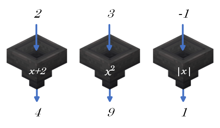
Feeding \(f\) a specific input like 3 is called evaluating \(f\) at 3, or informally "plugging 3 into \(f\)," and written \( f(3)\). To evaluate at an input, you just read through the algebraic expression defining the function, plugging in the input everywhere you see the variable. Take that middle example above. It's defined by \( f(x) = x^2\), with instructions "square that guy," so specifically \( f(3) = 3^2 = 9 \). Whatever appears in the box, \(f ( \textcolor{red}{\square})\), you slap in wherever the variable appears (often using parentheses!).
\[ f(\textcolor{red}{4}) = \textcolor{red}{4}^2, \quad \quad f(\textcolor{red}{a}) = \textcolor{red}{a}^2, \quad \quad f(\textcolor{red}{x-1}) = \textcolor{red}{(x-1)}^2 \notag \]
For the following functions, describe in words what the instructions are, and then evaluate at the given inputs.
- \( f(x) = x^2 + 1 \), at \(x = 0, 1, -2, 3x \)
- \( g(x) = \sqrt{x} \), at \(x = 1, 4, 9, x^2\)
- \( h(t) = 14 - 3t \), at \(t = 0, 4, 5, a-1 \)
Solution
1. The instructions are, "square the input and then add 1 to the result." Evaluations:
\[ f(0) = 0^2 + 1 = 1, \quad f(1) = 1^2 + 1 = 2, \quad f(-2) = (-2)^2 + 1 = 5, \quad f(3x) = (3x)^2 + 1 = 9x^2 + 1 \notag \]
2. The instructions are, "take the square root of the input." Evaluations:
\[ g(1) = \sqrt{1} = 1, \quad g(4) = \sqrt{4} = 2, \quad g(9) = \sqrt{9} = 3, \quad f(x^2) = \sqrt{x^2} = |x| \notag \]
3. The instructions are "multiply the input by 3, and then subtract the result from 14." Evaluations:
\[ h(0) = 14 - 3(0) = 14, \quad h(4) = 14 - 3(4) = 2, \quad h(5) = 14 - 3(5) = -1, \quad h(a-1) = 14 - 3(a-1) = 17 - 3a \notag \]
For the following functions, describe in words what the instructions are, and then evaluate at the given inputs.
- \( f(x) = (x-3)^3 \), at \(x = 1, 2, \star \)
- \( g(u) = \dfrac{u+2}{3} \), at \(u = -2, 0, 4, 2u\)
- \( h(t) = |t| \), at \(t = -3, 0, 3, t+1 \)
- Answer
-
1. "Subtract 3 from the input, then cube the result." Evaluations: \( f(1) = -8, f(2) = -1, f(\star) = (\star - 3)^3 \)
2. "Add 2 to the input, then divide the result by 3." Evaluations: \( g(-2) = 0, g(0) = \frac{2}{3}, g(4) = 2, g(2u) = \frac{2u+2}{3} \)
3. "Take the absolute value of the input." Evaluations: \( h(-3) = 3, h(0) = 0, h(3) = 0, h(t+1) = |t+1| \)
Functions From Tables
One way to give information about assigning outputs to inputs is with a table of values.
| \(x\) | \(f(x)\) |
| 0 | 0 |
| 1 | 1 |
| 2 | 4 |
| 3 | 9 |
| 4 | 16 |
| 5 | 25 |
Can you tell what definition of \(f\) would make sense from this table? Yeah, \(f(x) = x^2 \) would be consistent.
Guess the function's definition if the following table shows the outputs assigned to various inputs.
| \( x\) | \( f(x) \) |
| \( 0 \) | \( 1\) |
| \( 1\) | \( \dfrac{1}{2}\) |
| \( 2 \) | \( \dfrac{1}{3} \) |
| \( 5 \) | \(\dfrac{1}{6} \) |
| \( 10 \) | \( \dfrac{1}{11} \) |
| \( 100 \) | \( \dfrac{1}{101} \) |
- Answer
-
Looks like the function should be \(f(x) = \dfrac{1}{x+1} \). That would be a way to consistently get the desired outputs to come from the indicated inputs.
A key feature of the definition of a function is that it assigns exactly one output to each input! There can be no ambiguity about what will happen to an input. There's no way to give a function a single input and have two different options of output!
Based on what I just yelled about, why can't the table below define a function?
| inputs | outputs |
| \( 1\) | \(2\) |
| \( 2\) | \(3\) |
| \( 7\) | \( 12\) |
| \( 2\) | \(11\) |
| \( 9\) | \(15\) |
- Answer
-
Look at that sneaky row saying that \(2\) goes with \(11\) even though earlier it said \(2\) goes with \(3\)! This can't be a function, because it's assigned two different outputs to the same input. Illegal!
Functions as Maps
You could also imagine a function as a map that directs you from Input Land to Output Land by some rules. In this sense, the function is a bunch of arrows telling you where to send each input.

This sense of a function lets us visualize the "exactly one output for each input" rule mentioned above.

It's A-OK to assign two inputs to the same output, but it's illegal to send a single input to two different outputs. That would give \(f\) an existential crisis anytime you asked him to do anything. Can't have that.
This type of visualization of a function as a map will serve us well when we talk about compositions, so that's why I wanted you to see it here.
Functions From Graphs
Since a function assigns an output to each input, we could name the input \(x\) and name the output \(y\), and write them in a little pair together, \( (x,y)\). Ope, that looks familiar?? It looks like the coordinates of a point in the 2D plane! In the next section, we will learn how to draw graphs of functions, but for now let's connect the ideas basically.
Consider the function \(f(x) = x + 3 \). If we nickname the output \( f(x) \) as "\(y\)," suddenly we have the equation of a line in the coordinate plane, \(y = x+3\). For any input \(x\) we feed to \(f\), the output will give us a \(y\)-value that goes with that \(x\)-value on the line! That is, we have \( f(0) = 3\), and the point \( (0,3)\) is on the line. Similarly, \(f(1) = 4\), and the point \( (1,4) \) is on the line. For any input \(x\), the \(y\)-coordinate will be defined using \(f\) to be \(x+3\). In this scenario, the function value depends on the input \(x\), so \(x\) is the independent variable measured on the horizontal axis, and the function value output is telling us the value of the dependent variable measured on the vertical axis.

Going the other direction, let's try to express a function who describes the graph below.

I'm looking for a function to define the \(y\)-values, \(y = f(x) = \)???, to match all the points on this line. I could write these and similar points in a table like this:
| \(x\) | \(y = f(x)\) |
| \(0\) | \(-2\) |
| \(1\) | \(0\) |
| \(2\) | \(2\) |
| \(3\) | \(4\) |
Nice. I'd like to find the algebraic expression that defines the rule. It will not surprise me if it turns out to look like a linear equation, something in the form \(ax + b\), because my graph is a straight line. I see a \(y\)-intercept of \(-2\), and for every step to the right I take, I take two steps up. Rise-over-run-wise, that's a slope of positive 2. Maybe \(f(x) = 2x - 2\) will work? Confirm using the table and the picture that every point \( (x,y) \) on the line would satisfy this function definition...
\[ x = 0 \: \longrightarrow \: f(0) = -2 \checkmark, \quad x = 2 \: \longrightarrow \: f(2) = 2 \checkmark, \quad ... \notag \]
Try to identify the algebraic expression definition of the function whose graph is shown below.

- Answer
-
\( f(x) = -x + 3 \) will be satisfied by all points on the line, \( (x,y) = (x, f(x) )\), and matches the slope of \(-1\) and \(y\)-intercept of \(3\).
Domain Again
The domain of a function is the set of all inputs for the function. This may be explicitly given in a situation, such as
\[ f(x) = x + 4, \quad 0 \leq x \leq 20 \notag \]
or it may be implicitly assumed to be the domain of whatever algebraic expression is defining the function. In that case, the domain is whatever real numbers are legal to be plugged in for \(x\). Finally, in a real-world application problem, you should assess the domain by only including values that make sense in context.
It's often easier to talk about what isn't in the domain than what is...like it's usually a shorter list. When I ask you about domain, you will always say to yourself, "Self? What problem children will cause legality issues if I evaluate the function there?" This is exactly the same as analyzing the domain of an algebraic expression. We report our answers the same way: with interval notation, words, set notation, whatever as long as it's clear, communicative, and true.
Find the domains of the functions given.
- \(p(x) = x^2 + 2 \)
- \( g(x) = \dfrac{1}{x} \)
- \( h(t) = 12 - \sqrt{t} \)
- \( f(n) = \dfrac{2}{\sqrt{n+2}} \)
- \( V(x) = x^2(30-x) \), which gives the volume of a certain box with square base, dependent on the side length of the base, \(x\).
Solution
- This function is defined using a polynomial, and everything is legal to plug into polynomials. I'm always looking out for two things: dividing by zero, and taking square roots of negative numbers. Neither is an issue here. The domain is thus all real numbers, written \( \mathbb{R}\) or in interval notation, \(( -\infty, \infty)\). Note: this is not a coordinate point, it's an open interval!
- This function has division involved, so we cannot allow \(x\) to be 0. We say "all real numbers, \(x \neq 0\)," or maybe \( (-\infty, 0) \cup (0, \infty)\), or maybe \( \{x \: | \: x \neq 0\} \).
- This function has a square root, so I can't plug in any negative numbers for \(t\). We say, "all nonnegative real numbers," or \( [0, \infty) \), etc.
- This function has division and square roots! First of all, I can't let \(n\) be anything that would cause the inside of the square root to be negative. Aka, I must require that \( n+2 \geq 0\). By solving the inequality, I see this is guaranteed if \(n \geq -2\). BUT I also can't divide by zero, and if \(n = -2\), that happens. :( So I can't allow \(-2\) in my domain either. My final answer is \( n > -2\), or \( (-2,\infty)\).
- This describes a physical quantity, so we think about what answers would be silly. It won't be much of a box if its base has dimensions \(0 \times 0\), so we could restrict \(x > 0\). It also doesn't make sense to have a negative dimension or negative volume, which would happen if \(x > 30 \) because of the \((30-x)\) factor. Since \(x = 30\) would also result in a volume of 0, I'd probably throw that out and say my domain of interest for this function is just \( 0 < x < 30 \).
Find the domains of the functions given.
- \( q(x) = (x+1)(x-1)(x+2) \)
- \( f(x) = \sqrt{2x-1} + 4 \)
- \( g(y) = \frac{y - 1}{y+3}\)
- \( A(r) = \pi r^2\), a function giving the area of a circle I plan to cut out of a 12in \( \times\) 20in rectangle of cardboard.
- Answer
-
- All real numbers.
- \( \left\{x \: | \: x \geq \frac{1}{2} \right\} \)
- \( y \neq -3\)
- It wouldn't make any sense to cut out a circle with negative radius, and I don't want a radius of zero (would that be just stabbing a pin through the cardboard??) so I'm going to restrict \(r > 0 \). But also, the smallest dimension of my cardboard is 12in, so even if I position the circle in the middle of the rectangle, I can't have a diameter larger than 12in. That restricts my radius to 6in max. The domain I'm interested in is \(0 < r \leq 6 \).