2.01: Prerequisites to Numerical Differentiation
- Page ID
- 126394
\( \newcommand{\vecs}[1]{\overset { \scriptstyle \rightharpoonup} {\mathbf{#1}} } \)
\( \newcommand{\vecd}[1]{\overset{-\!-\!\rightharpoonup}{\vphantom{a}\smash {#1}}} \)
\( \newcommand{\dsum}{\displaystyle\sum\limits} \)
\( \newcommand{\dint}{\displaystyle\int\limits} \)
\( \newcommand{\dlim}{\displaystyle\lim\limits} \)
\( \newcommand{\id}{\mathrm{id}}\) \( \newcommand{\Span}{\mathrm{span}}\)
( \newcommand{\kernel}{\mathrm{null}\,}\) \( \newcommand{\range}{\mathrm{range}\,}\)
\( \newcommand{\RealPart}{\mathrm{Re}}\) \( \newcommand{\ImaginaryPart}{\mathrm{Im}}\)
\( \newcommand{\Argument}{\mathrm{Arg}}\) \( \newcommand{\norm}[1]{\| #1 \|}\)
\( \newcommand{\inner}[2]{\langle #1, #2 \rangle}\)
\( \newcommand{\Span}{\mathrm{span}}\)
\( \newcommand{\id}{\mathrm{id}}\)
\( \newcommand{\Span}{\mathrm{span}}\)
\( \newcommand{\kernel}{\mathrm{null}\,}\)
\( \newcommand{\range}{\mathrm{range}\,}\)
\( \newcommand{\RealPart}{\mathrm{Re}}\)
\( \newcommand{\ImaginaryPart}{\mathrm{Im}}\)
\( \newcommand{\Argument}{\mathrm{Arg}}\)
\( \newcommand{\norm}[1]{\| #1 \|}\)
\( \newcommand{\inner}[2]{\langle #1, #2 \rangle}\)
\( \newcommand{\Span}{\mathrm{span}}\) \( \newcommand{\AA}{\unicode[.8,0]{x212B}}\)
\( \newcommand{\vectorA}[1]{\vec{#1}} % arrow\)
\( \newcommand{\vectorAt}[1]{\vec{\text{#1}}} % arrow\)
\( \newcommand{\vectorB}[1]{\overset { \scriptstyle \rightharpoonup} {\mathbf{#1}} } \)
\( \newcommand{\vectorC}[1]{\textbf{#1}} \)
\( \newcommand{\vectorD}[1]{\overrightarrow{#1}} \)
\( \newcommand{\vectorDt}[1]{\overrightarrow{\text{#1}}} \)
\( \newcommand{\vectE}[1]{\overset{-\!-\!\rightharpoonup}{\vphantom{a}\smash{\mathbf {#1}}}} \)
\( \newcommand{\vecs}[1]{\overset { \scriptstyle \rightharpoonup} {\mathbf{#1}} } \)
\(\newcommand{\longvect}{\overrightarrow}\)
\( \newcommand{\vecd}[1]{\overset{-\!-\!\rightharpoonup}{\vphantom{a}\smash {#1}}} \)
\(\newcommand{\avec}{\mathbf a}\) \(\newcommand{\bvec}{\mathbf b}\) \(\newcommand{\cvec}{\mathbf c}\) \(\newcommand{\dvec}{\mathbf d}\) \(\newcommand{\dtil}{\widetilde{\mathbf d}}\) \(\newcommand{\evec}{\mathbf e}\) \(\newcommand{\fvec}{\mathbf f}\) \(\newcommand{\nvec}{\mathbf n}\) \(\newcommand{\pvec}{\mathbf p}\) \(\newcommand{\qvec}{\mathbf q}\) \(\newcommand{\svec}{\mathbf s}\) \(\newcommand{\tvec}{\mathbf t}\) \(\newcommand{\uvec}{\mathbf u}\) \(\newcommand{\vvec}{\mathbf v}\) \(\newcommand{\wvec}{\mathbf w}\) \(\newcommand{\xvec}{\mathbf x}\) \(\newcommand{\yvec}{\mathbf y}\) \(\newcommand{\zvec}{\mathbf z}\) \(\newcommand{\rvec}{\mathbf r}\) \(\newcommand{\mvec}{\mathbf m}\) \(\newcommand{\zerovec}{\mathbf 0}\) \(\newcommand{\onevec}{\mathbf 1}\) \(\newcommand{\real}{\mathbb R}\) \(\newcommand{\twovec}[2]{\left[\begin{array}{r}#1 \\ #2 \end{array}\right]}\) \(\newcommand{\ctwovec}[2]{\left[\begin{array}{c}#1 \\ #2 \end{array}\right]}\) \(\newcommand{\threevec}[3]{\left[\begin{array}{r}#1 \\ #2 \\ #3 \end{array}\right]}\) \(\newcommand{\cthreevec}[3]{\left[\begin{array}{c}#1 \\ #2 \\ #3 \end{array}\right]}\) \(\newcommand{\fourvec}[4]{\left[\begin{array}{r}#1 \\ #2 \\ #3 \\ #4 \end{array}\right]}\) \(\newcommand{\cfourvec}[4]{\left[\begin{array}{c}#1 \\ #2 \\ #3 \\ #4 \end{array}\right]}\) \(\newcommand{\fivevec}[5]{\left[\begin{array}{r}#1 \\ #2 \\ #3 \\ #4 \\ #5 \\ \end{array}\right]}\) \(\newcommand{\cfivevec}[5]{\left[\begin{array}{c}#1 \\ #2 \\ #3 \\ #4 \\ #5 \\ \end{array}\right]}\) \(\newcommand{\mattwo}[4]{\left[\begin{array}{rr}#1 \amp #2 \\ #3 \amp #4 \\ \end{array}\right]}\) \(\newcommand{\laspan}[1]{\text{Span}\{#1\}}\) \(\newcommand{\bcal}{\cal B}\) \(\newcommand{\ccal}{\cal C}\) \(\newcommand{\scal}{\cal S}\) \(\newcommand{\wcal}{\cal W}\) \(\newcommand{\ecal}{\cal E}\) \(\newcommand{\coords}[2]{\left\{#1\right\}_{#2}}\) \(\newcommand{\gray}[1]{\color{gray}{#1}}\) \(\newcommand{\lgray}[1]{\color{lightgray}{#1}}\) \(\newcommand{\rank}{\operatorname{rank}}\) \(\newcommand{\row}{\text{Row}}\) \(\newcommand{\col}{\text{Col}}\) \(\renewcommand{\row}{\text{Row}}\) \(\newcommand{\nul}{\text{Nul}}\) \(\newcommand{\var}{\text{Var}}\) \(\newcommand{\corr}{\text{corr}}\) \(\newcommand{\len}[1]{\left|#1\right|}\) \(\newcommand{\bbar}{\overline{\bvec}}\) \(\newcommand{\bhat}{\widehat{\bvec}}\) \(\newcommand{\bperp}{\bvec^\perp}\) \(\newcommand{\xhat}{\widehat{\xvec}}\) \(\newcommand{\vhat}{\widehat{\vvec}}\) \(\newcommand{\uhat}{\widehat{\uvec}}\) \(\newcommand{\what}{\widehat{\wvec}}\) \(\newcommand{\Sighat}{\widehat{\Sigma}}\) \(\newcommand{\lt}{<}\) \(\newcommand{\gt}{>}\) \(\newcommand{\amp}{&}\) \(\definecolor{fillinmathshade}{gray}{0.9}\)Lesson 1: Prerequisites to Numerical Differentiation
Learning Objectives
After successful completion of this lesson, you should be able to:
1) recall the exact definition of differentiation
2) derive exact derivatives of a few functions
Introduction
In this lesson, we will review the necessary concepts of differential calculus to learn numerical differentiation. These include the concepts of finding exact derivatives of functions.
The derivative of a function represents the rate of change of a variable with respect to another variable. For example, the velocity of a body is defined as the rate of change of the location of the body with respect to time. The location is the dependent variable, while time is the independent variable. Now, if we measure the rate of change of velocity with respect to time, we get the acceleration of the body. In this case, velocity is the dependent variable, while time is the independent variable.
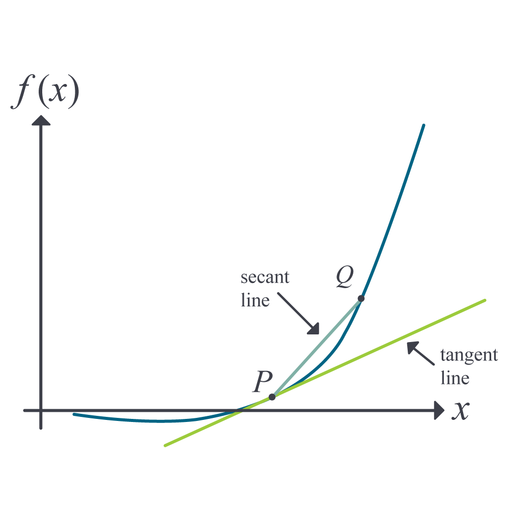
Whenever differentiation is introduced to a student, the two concepts of the secant line and tangent line (Figure \(\PageIndex{1.1}\)) are revisited.

Let \(P\) and \(Q\) be two points on the curve, as shown in Figure 1. The secant line is the straight line drawn through \(P\) and \(Q\).

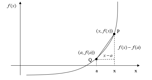
The slope of the secant line (Figure \(\PageIndex{1.2})\) is then given as
\[\begin{split} m_{PQ, secant} &= \frac{f(a + h) - f(a)}{(a + h) - a}\\ &=\frac{f(a + h) - f(a)}{h}\end{split} \;\;\;\;\;\;\;\;\;\;\;\; (\PageIndex{1.1}) \nonumber\]
As \(Q\) moves closer and closer to \(P\), the limiting portion is called the tangent line. The slope of the tangent line \(m_{PQ, tangent}\) then is the limiting value of \(m_{PQ, secant}\) from Equation \((\PageIndex{1.1})\) as \(h \rightarrow 0\).
\[m_{PQ, tangent} = \lim_{h \rightarrow 0}\frac{f(a + h) - f(a)}{h} \;\;\;\;\;\;\;\;\;\;\;\; (\PageIndex{1.2}) \nonumber\]
Find the slope of the secant line of the curve \(y = 4x^{2}\) between points \((3,36)\) and \((5,100)\).
Solution
The slope of the secant line between \((3,36)\) and \((5,100)\) from Equation \((\PageIndex{1.1})\) is
\[\begin{split} m &=\frac{f(5) - f(3)}{5 - 3}\\ &=\frac{100 - 36}{5 - 3}\\ &= 32\end{split} \nonumber\]
Find the slope of the tangent line of the curve \(y = 4x^{2}\) at point \((3,36)\).
Solution
The slope of the tangent line at \((3,36)\) from Equation \((\PageIndex{1.2})\) is \[\begin{split} m &= \lim_{h \rightarrow 0}\frac{f(3 + h) - f(3)}{h}\\ &= \lim_{h \rightarrow 0}\frac{4(3 + h)^{2} - 4(3)^{2}}{h}\\ &= \lim_{h \rightarrow 0}\frac{4(9 + h^{2} + 6h) - 36}{h}\\ &= \lim_{h \rightarrow 0}\frac{36 + 4h^{2} + 24h - 36}{h}\\ &= \lim_{h \rightarrow 0}\frac{h(4h + 24)}{h}\\ &= \lim_{h \rightarrow 0}(4h + 24)\\ &= 24\end{split} \nonumber\]

Derivative of a Function
Recall from calculus, the derivative of a function \(f(x)\) at \(x = a\) is defined as the slope of the tangent line at \(x = a\)
\[f^{\prime}(a) = \lim_{h \rightarrow 0}\frac{f(a + h) - f(a)}{h} \;\;\;\;\;\;\;\;\;\;\;\; (\PageIndex{1.3}) \nonumber\]
Find \(f^{\prime}(3)\) if \(f(x) = 4x^{2}\).
Solution
\[\begin{split} f^{\prime}(x) &= 4(2x)\\ &= 8x\\ &=24 \end{split} \nonumber\]

Second Definition of Derivatives
There is another form of the definition of the derivative of a function. The derivative of the function \(f(x)\) at \(x = a\) is defined as
\[f^{\prime}(a) = \lim_{x \rightarrow a}\frac{f(x) - f(a)}{x - a} \;\;\;\;\;\;\;\;\;\;\;\; (\PageIndex{1.4}) \nonumber\]
As \(x \rightarrow a\), the definition is nothing but the slope of the tangent line at \(P\).

Find \(f^{\prime}(3)\) if \(f(x) = 4x^{2}\) by using the form
\[f^{\prime}(a) = \lim_{x \rightarrow a}\frac{f(x) - f(a)}{x - a} \nonumber\]
of the definition of a derivative.
Solution
\[\begin{split} f^{\prime}(3) &= \lim_{x \rightarrow 3}\frac{f(x) - f(3)}{x - 3}\\ &= \lim_{x \rightarrow 3}\frac{4x^{2} - 4(3)^{2}}{x - 3}\\ &= \lim_{x \rightarrow 3}\frac{4x^{2} - 36}{x - 3}\\ &= \lim_{x \rightarrow 3}\frac{4(x^{2} - 9)}{x - 3}\\ &= \lim_{x \rightarrow 3}\frac{4(x - 3)(x + 3)}{x - 3}\\ &= \lim_{x \rightarrow 3}4(x + 3)\\ &= 4(3 + 3) \\ &= 24 \end{split} \nonumber\]
Higher-Order Derivatives
So far, we have limited our discussion to calculating the first derivative, \(f^{\prime}(x)\) of a function \(f(x)\). What if we are asked to calculate higher-order derivatives of \(f(x)\). A simple example of this is finding the acceleration of a body from a function that gives the location of the body as a function of time. The derivative of the location with respect to time is the velocity of the body, followed by the derivative of velocity with respect to time being the acceleration. Hence, the second derivative of the location function gives the acceleration function of the body.
Given \(f(x) = 3x^{3} - 2x - 7\), find the second derivative, \(f^{\prime\prime}(x)\), and the third derivative, \(f^{\prime\prime\prime}(x)\). Also, find the value of \(f^{\prime\prime}(2)\) and \(f^{\prime\prime\prime}(2)\).
Solution
Given
\[f(x) = 3x^{3} - 2x - 7 \nonumber\]
we have
\[\begin{split} f^{\prime}(x) &= 3(3x^{2}) - 2\\ &= 9x^{2} - 2\end{split} \nonumber\]
\[\begin{split} f^{\prime\prime}(x) &= \frac{d}{dx}(f^{\prime}(x))\\ &= \frac{d}{dx}\left( 9x^{2} - 2 \right)\\ &= 9\left( 2x \right)\\ &= 18x\end{split}\nonumber \]
\[\begin{split} f\left( 2 \right) &= 18 \times 2\\ &= 36 \end{split} \nonumber\]
\[\begin{split} f^{\prime\prime\prime}(x) &= \frac{d}{dx}(f^{\prime\prime}(x))\\ &= \frac{d}{dx}(18x)\\ &= 18\end{split} \nonumber\]
\[f^{\prime\prime\prime}(2) = 18 \nonumber\]
Other Notations of Derivatives
Derivatives can be denoted in several ways. For the first derivative, the notations include
\[f^{\prime}(x),\ \frac{d}{dx}f(x),\ y^{\prime}, \dot{y},\ \text{and}\ \frac{dy}{dx} \nonumber\]
For the second derivative, the notations include
\[f^{\prime\prime}(x),\ \frac{d^{2}}{dx^{2}}f(x),\ y^{\prime\prime},\ \ddot{y},\ \text{and}\ \frac{d^{2}y}{dx^{2}} \nonumber\]
For the \(n^{th}\) derivative, the notations include
\[f^{(n)}(x),\ \frac{d^{n}}{dx^{n}}f(x),\ y^{(n)},\ \text{and}\ \frac{d^{n}y}{dx^{n}} \nonumber\]
Lesson 2: Equation of a Tangent Line
Learning Objectives
After successful completion of this lesson, you should be able to:
1) find the equation of the tangent line to a function.
Finding equations of a tangent line
One of the numerical methods used to solve a nonlinear equation is called the Newton-Raphson method. This method is based on the prerequisite knowledge of finding the tangent line to a curve at a point. Let us look at an example to illustrate finding the equation of the tangent line to a curve.
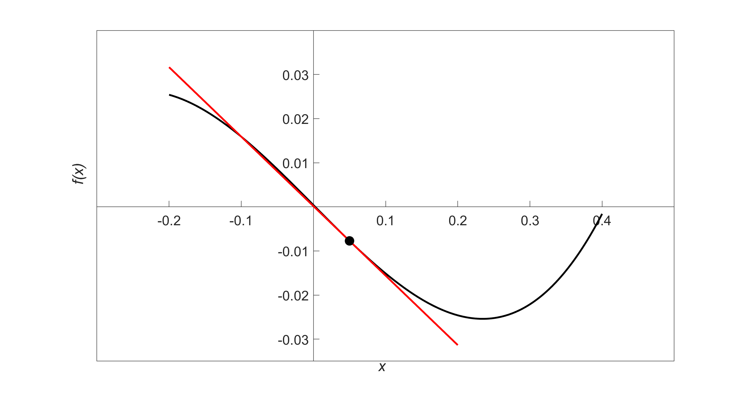
Find the equation of the line tangent to the function
\[f(x) = x^{3} - 0.165x + 3.993 \times 10^{- 4} \nonumber\]
at \(x = 0.05.\)
Solution
The line tangent is a straight line of the form
\[y = mx + c \nonumber\]
To find the equation of the tangent line, let us first find the slope \(m\) of the straight line.
\[f^{\prime}(x) = 3x^{2} - 0.165 \nonumber\]
At \(x=0.05\)\[\begin{split} f^{\prime}(0.05) &= 3(0.05)^{2} - 0.165\\ &= - 0.1575 \end{split} \nonumber\]
Hence\[m = - 0.1575 \nonumber\]
To find the value of the \(y\)-intercept \(c\) of the straight line, we first find the value of the function at \(x = 0.05\).
\[\begin{split} f(0.05) &= (0.05)^{3} - 0.165(0.05) + 3.993 \times 10^{- 4}\\ &= - 0.0077257 \end{split} \nonumber\]
The tangent line passes through the point \((0.05, - 0.0077257)\), so
\[- 0.0077257 = m(0.05) + c \nonumber\]
\[- 0.0077257 = - 0.1575(0.05) + c \nonumber\]
\[c = 0.0001493 \nonumber\]

Hence,
\[\begin{split} y &= mx + c\\ &= - 0.1575x + 0.0001493 \end{split} \nonumber\]
is the equation of the tangent line.
Multiple Choice Test
(1). The definition of the first derivative of a function \(f(x)\) is
(A) \(\displaystyle f^{\prime}(x) = \frac{f(x + \Delta x) + f(x)}{\Delta x}\)
(B) \(\displaystyle f^{\prime}(x) = \frac{f(x + \Delta x) - f(x)}{\Delta x}\)
(C) \(\displaystyle f^{\prime}(x) = \lim_{\Delta x \rightarrow 0} \frac{f(x + \Delta x) + f(x)}{\Delta x}\)
(D) \(\displaystyle f^{\prime}(x) = \lim_{\Delta x \rightarrow 0}\frac{f(x + \Delta x) - f(x)}{\Delta x}\)
(2). Given \(y = 5e^{3x} + \sin x\), \(\displaystyle \frac{dy}{dx}\) is
(A) \(5e^{3x} + \cos x\)
(B) \(15e^{3x} + \cos x\)
(C) \(15e^{3x} - \cos x\)
(D) \(2.666e^{3x} - \cos x\)
(3). Given \(y = \sin 2x\), \(\displaystyle \frac{dy}{dx}\) at \(x = 3\) is most nearly
(A) \(0.9600\)
(B) \(0.9945\)
(C) \(1.920\)
(D) \(1.989\)
(4). Given \(y = x^{3}\ln x\), \(\displaystyle \frac{dy}{dx}\) is
(A) \(3x^{2}\ln x\)
(B) \(3x^{2}\ln x + x^{2}\)
(C) \(x^{2}\)
(D) \(3x\)
(5). The velocity of a body as a function of time is given as \(v\left( t \right) = 5e^{- 2t} + 4\), where \(t\) is in seconds, and \(v\) is in m/s. The acceleration in \(\text{m} / \text{s}^{2}\) at \(t = 0.6 \ \text{s}\) is
(A) \(-3.012\)
(B) \(5.506\)
(C) \(4.147\)
(D) \(-10.00\)
(6). If \(x^{2} + 2xy = y^{2}\), then \(\displaystyle \frac{dy}{dx}\) is
(A) \(\displaystyle \frac{x + y}{y - x}\)
(B) \(2x + 2y\)
(C) \(\displaystyle \frac{x + 1}{y}\)
(D) \(- x\)
For complete solution, go to
http://nm.mathforcollege.com/mcquizzes/02dif/quiz_02dif_background_solution.pdf


