
2.03: Numerical Differentiation of Functions at Discrete Data Points
- Page ID
- 126396
\( \newcommand{\vecs}[1]{\overset { \scriptstyle \rightharpoonup} {\mathbf{#1}} } \)
\( \newcommand{\vecd}[1]{\overset{-\!-\!\rightharpoonup}{\vphantom{a}\smash {#1}}} \)
\( \newcommand{\dsum}{\displaystyle\sum\limits} \)
\( \newcommand{\dint}{\displaystyle\int\limits} \)
\( \newcommand{\dlim}{\displaystyle\lim\limits} \)
\( \newcommand{\id}{\mathrm{id}}\) \( \newcommand{\Span}{\mathrm{span}}\)
( \newcommand{\kernel}{\mathrm{null}\,}\) \( \newcommand{\range}{\mathrm{range}\,}\)
\( \newcommand{\RealPart}{\mathrm{Re}}\) \( \newcommand{\ImaginaryPart}{\mathrm{Im}}\)
\( \newcommand{\Argument}{\mathrm{Arg}}\) \( \newcommand{\norm}[1]{\| #1 \|}\)
\( \newcommand{\inner}[2]{\langle #1, #2 \rangle}\)
\( \newcommand{\Span}{\mathrm{span}}\)
\( \newcommand{\id}{\mathrm{id}}\)
\( \newcommand{\Span}{\mathrm{span}}\)
\( \newcommand{\kernel}{\mathrm{null}\,}\)
\( \newcommand{\range}{\mathrm{range}\,}\)
\( \newcommand{\RealPart}{\mathrm{Re}}\)
\( \newcommand{\ImaginaryPart}{\mathrm{Im}}\)
\( \newcommand{\Argument}{\mathrm{Arg}}\)
\( \newcommand{\norm}[1]{\| #1 \|}\)
\( \newcommand{\inner}[2]{\langle #1, #2 \rangle}\)
\( \newcommand{\Span}{\mathrm{span}}\) \( \newcommand{\AA}{\unicode[.8,0]{x212B}}\)
\( \newcommand{\vectorA}[1]{\vec{#1}} % arrow\)
\( \newcommand{\vectorAt}[1]{\vec{\text{#1}}} % arrow\)
\( \newcommand{\vectorB}[1]{\overset { \scriptstyle \rightharpoonup} {\mathbf{#1}} } \)
\( \newcommand{\vectorC}[1]{\textbf{#1}} \)
\( \newcommand{\vectorD}[1]{\overrightarrow{#1}} \)
\( \newcommand{\vectorDt}[1]{\overrightarrow{\text{#1}}} \)
\( \newcommand{\vectE}[1]{\overset{-\!-\!\rightharpoonup}{\vphantom{a}\smash{\mathbf {#1}}}} \)
\( \newcommand{\vecs}[1]{\overset { \scriptstyle \rightharpoonup} {\mathbf{#1}} } \)
\(\newcommand{\longvect}{\overrightarrow}\)
\( \newcommand{\vecd}[1]{\overset{-\!-\!\rightharpoonup}{\vphantom{a}\smash {#1}}} \)
\(\newcommand{\avec}{\mathbf a}\) \(\newcommand{\bvec}{\mathbf b}\) \(\newcommand{\cvec}{\mathbf c}\) \(\newcommand{\dvec}{\mathbf d}\) \(\newcommand{\dtil}{\widetilde{\mathbf d}}\) \(\newcommand{\evec}{\mathbf e}\) \(\newcommand{\fvec}{\mathbf f}\) \(\newcommand{\nvec}{\mathbf n}\) \(\newcommand{\pvec}{\mathbf p}\) \(\newcommand{\qvec}{\mathbf q}\) \(\newcommand{\svec}{\mathbf s}\) \(\newcommand{\tvec}{\mathbf t}\) \(\newcommand{\uvec}{\mathbf u}\) \(\newcommand{\vvec}{\mathbf v}\) \(\newcommand{\wvec}{\mathbf w}\) \(\newcommand{\xvec}{\mathbf x}\) \(\newcommand{\yvec}{\mathbf y}\) \(\newcommand{\zvec}{\mathbf z}\) \(\newcommand{\rvec}{\mathbf r}\) \(\newcommand{\mvec}{\mathbf m}\) \(\newcommand{\zerovec}{\mathbf 0}\) \(\newcommand{\onevec}{\mathbf 1}\) \(\newcommand{\real}{\mathbb R}\) \(\newcommand{\twovec}[2]{\left[\begin{array}{r}#1 \\ #2 \end{array}\right]}\) \(\newcommand{\ctwovec}[2]{\left[\begin{array}{c}#1 \\ #2 \end{array}\right]}\) \(\newcommand{\threevec}[3]{\left[\begin{array}{r}#1 \\ #2 \\ #3 \end{array}\right]}\) \(\newcommand{\cthreevec}[3]{\left[\begin{array}{c}#1 \\ #2 \\ #3 \end{array}\right]}\) \(\newcommand{\fourvec}[4]{\left[\begin{array}{r}#1 \\ #2 \\ #3 \\ #4 \end{array}\right]}\) \(\newcommand{\cfourvec}[4]{\left[\begin{array}{c}#1 \\ #2 \\ #3 \\ #4 \end{array}\right]}\) \(\newcommand{\fivevec}[5]{\left[\begin{array}{r}#1 \\ #2 \\ #3 \\ #4 \\ #5 \\ \end{array}\right]}\) \(\newcommand{\cfivevec}[5]{\left[\begin{array}{c}#1 \\ #2 \\ #3 \\ #4 \\ #5 \\ \end{array}\right]}\) \(\newcommand{\mattwo}[4]{\left[\begin{array}{rr}#1 \amp #2 \\ #3 \amp #4 \\ \end{array}\right]}\) \(\newcommand{\laspan}[1]{\text{Span}\{#1\}}\) \(\newcommand{\bcal}{\cal B}\) \(\newcommand{\ccal}{\cal C}\) \(\newcommand{\scal}{\cal S}\) \(\newcommand{\wcal}{\cal W}\) \(\newcommand{\ecal}{\cal E}\) \(\newcommand{\coords}[2]{\left\{#1\right\}_{#2}}\) \(\newcommand{\gray}[1]{\color{gray}{#1}}\) \(\newcommand{\lgray}[1]{\color{lightgray}{#1}}\) \(\newcommand{\rank}{\operatorname{rank}}\) \(\newcommand{\row}{\text{Row}}\) \(\newcommand{\col}{\text{Col}}\) \(\renewcommand{\row}{\text{Row}}\) \(\newcommand{\nul}{\text{Nul}}\) \(\newcommand{\var}{\text{Var}}\) \(\newcommand{\corr}{\text{corr}}\) \(\newcommand{\len}[1]{\left|#1\right|}\) \(\newcommand{\bbar}{\overline{\bvec}}\) \(\newcommand{\bhat}{\widehat{\bvec}}\) \(\newcommand{\bperp}{\bvec^\perp}\) \(\newcommand{\xhat}{\widehat{\xvec}}\) \(\newcommand{\vhat}{\widehat{\vvec}}\) \(\newcommand{\uhat}{\widehat{\uvec}}\) \(\newcommand{\what}{\widehat{\wvec}}\) \(\newcommand{\Sighat}{\widehat{\Sigma}}\) \(\newcommand{\lt}{<}\) \(\newcommand{\gt}{>}\) \(\newcommand{\amp}{&}\) \(\definecolor{fillinmathshade}{gray}{0.9}\)Lesson 1: Numerical Differentiation of Functions Given as Discrete Data Points - First Derivative
Lesson Objectives
After successful completion of this lesson, you should be able to:
1) choose the most proper scheme among FDD, BDD, and CDD based on order of accuracy and data availability,
2) find numerical values of the first derivatives of functions that are given at discrete data points.
Introduction
To find the derivatives of functions that are given at discrete points, several methods are available. Although these methods are mainly used when the data is spaced unequally, they can be used for data that is spaced equally as well.
We know
\[f^{\prime}\left( x \right) = \lim_{\Delta x \rightarrow 0}\frac{f\left( x + \Delta x \right) - f\left( x \right)}{\Delta x} \nonumber\]
We developed finite divided difference approximations for the first and second derivatives of continuous functions in a previous lesson. We can apply the same formulas for discrete functions as well. However, some limitations exist, and one should note them before applying any of the approximations.
So given \(n + 1\) data points in ascending order of \(x\) values, \(\left( x_{0},y_{0} \right), \ \left( x_{1},y_{1} \right), \ \left( x_{2},y_{2} \right),\ldots,\left( x_{n},y_{n} \right)\), the value of \(f^{\prime}(x_i)\) by FDD for \(x_{i} \leq x \leq x_{i + 1}\), \(i = 0,...,n - 1\), is given by
\[f^{\prime}\left( x_{i} \right) \approx \frac{f\left( x_{i + 1} \right) - f\left( x_{i} \right)}{x_{i + 1} - x_{i}}\;\;\;\;\;\;\;\;\;\;\;\; (\PageIndex{1.1}) \nonumber\]
the value of \(f^{\prime}(x_i)\) by BDD for \(x_{i - 1} \leq x \leq x_{i}\), \(i = 1,...,n\), is given by
\[f^{\prime}\left( x_{i} \right) \approx \frac{f\left( x_{i} \right) - f\left( x_{i - 1} \right)}{x_{i} - x_{i - 1}}\;\;\;\;\;\;\;\;\;\;\;\; (\PageIndex{1.2}) \nonumber\]
the value of \(f^{\prime}(x_i)\) by CDD for \(x_{i - 1} \leq x \leq x_{i + 1}\), \(i = 1,...,n - 1\), is given by
\[f^{\prime}\left( x_{i} \right) \approx \frac{f\left( x_{i + 1} \right) - f\left( x_{i - 1} \right)}{x_{i + 1} - x_{i - 1}}\;\;\;\;\;\;\;\;\;\;\;\;(\PageIndex{1.3}) \nonumber\]
provided that \[x_{i + 1} - x_{i} = x_{i} - x_{i - 1}. \nonumber\]
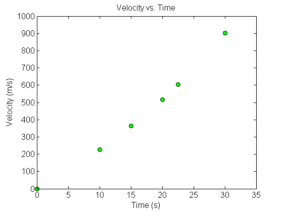
The upward velocity of a rocket is given as a function of time in Table \(\PageIndex{1.1}\).
| \(t\ \text{(s)}\) | \(v(t)\ (\text{m/s})\) |
|---|---|
| \(0\) | \(0\) |
| \(10\) | \(227.04\) |
| \(15\) | \(362.78\) |
| \(20\) | \(517.35\) |
| \(22.5\) | \(602.97\) |
| \(30\) | \(901.67\) |
a) Use forward divided difference, if possible, to find the acceleration of the rocket at \(t = 15\text{ s}\).
b) Use backward divided difference, if possible, to find the acceleration of the rocket at \(t = 15\text{ s}\).
c) Use central divided difference, if possible, to find the acceleration of the rocket at \(t = 15\text{ s}\).
Solution
a) To find the acceleration at \(t = 15\text{ s}\) with the forward divided difference method, a data point ahead of \(t = 15\text{ s}\) should be available. All these conditions are met, and we will use velocity values at \(t = 15\text{ s}\) and \(t = 20\text{ s}\)
\[a\left( t_{i} \right) \approx \frac{v\left( t_{i + 1} \right) - v\left( t_{i} \right)}{t_{i+1}-t_i} \nonumber\]
\[t_{i} = 15 \nonumber\]
\[t_{i + 1} = 20 \nonumber\]
\[\begin{split} a\left( 15 \right) &\approx \frac{v\left( 20 \right) - v\left( 15 \right)}{20-15}\\\\ &= \frac{517.35 - 362.78}{5}\\\\ &=30.914\ \text{m/s}^{2}\end{split} \nonumber\]
b) To find the acceleration at \(t = 15\text{ s}\) with the backward divided difference method, a data point behind \(t = 15 \text{ s}\) should be available. All these conditions are met, and we will use velocity values at \(t = 10\text{ s}\) and \(t = 15\text{ s}\)
\[a\left( t_{i} \right) \approx \frac{v\left( t_{i} \right) - v\left( t_{i - 1} \right)}{t_i-t_{i-1}} \nonumber\]
\[t_{i - 1} = 10 \nonumber\]
\[t_{i} = 15 \nonumber\]
\[\begin{split} a\left( 15 \right) &\approx \frac{v\left( 15 \right) - v\left( 10 \right)}{15-10}\\\\ &= \frac{362.78 - 227.04}{5}\\\\ &=27.148 \text{ m/s}^{2}\end{split} \nonumber\]
c) To find the acceleration at \(t = 15\text{ s}\) with the central divided difference method,
- a data point behind \(t = 15\text{ s}\) should be available,
- a data point ahead of \(t = 15\text{ s}\) should be available, and
- the spacing should be the same on the time domain from \(t = 15\text{ s}\).
All these conditions are met, and we will use velocity values at \(t = 10\text{ s}\) and \(t = 20\text{ s}\)
\[a\left( t_{i} \right) \approx \frac{v\left( t_{i + 1} \right) - v\left( t_{i - 1} \right)}{t_{i+1}-t_{i-1}} \nonumber\]
\[t_{i - 1} = 10 \nonumber\]
\[t_{i + 1} = 20 \nonumber\]
\[\begin{split} a\left( 15 \right) &\approx \frac{v\left( 20 \right) - v\left( 10 \right)}{20-10}\\\\ &= \frac{517.35 - 227.04}{10}\\\\ &={29.031 \text{ m/s}^{2}}\end{split} \nonumber\]
The values of acceleration at \(t=15 \text{ s}\) obtained using the three divided difference schemes is given in Table \(\PageIndex{1.2}\).
| Method | \(a(15)\text{ (m/s}^{2})\) |
|---|---|
| Forward | \(30.914\) |
| Backward | \(27.148\) |
| Central | \(29.031\) |
Lesson 2: Numerical Differentiation of Functions Given as Discrete Data Points - Second Derivative
Learning Objectives
After successful completion of this lesson, you should be able to:
1) find approximate values of the second derivatives of functions that are given at discrete data points
Introduction
To find the derivatives of functions that are given at discrete points, several methods are available. Although these methods are mainly used when the data is spaced unequally, they can be used for data spaced equally.
In a previous lesson, we developed finite divided difference approximations for the second derivatives of continuous functions. We can apply the same formulas for discrete functions as well. However, some limitations exist, and one should note them before applying any of the approximations.
So given \(n + 1\) data points in ascending order of \(x\) values, \(\left( x_{0},y_{0} \right), \ \left( x_{1},y_{1} \right), \ \left( x_{2},y_{2} \right),\ldots,\left( x_{n},y_{n} \right)\),
the value of \(f^{\prime\prime}(x_{i})\) by CDD for \(x_{i - 1} \leq x_{i} \leq x_{i + 1}\), \(i = 1,\ldots,n - 1\), is given by
\[f^{\prime\prime}\left( x_{i} \right) \approx \frac{f\left( x_{i + 1} \right) - 2f\left( x_{i} \right) + f\left( x_{i - 1} \right)}{(x_{i + 1} - x_{i})^{2}} \nonumber\]
provided that \[x_{i + 1} - x_{i} = x_{i} - x_{i - 1}. \nonumber\]
The upward velocity of a rocket is given as a function of time in Table \(\PageIndex{2.1}\).
| \(t\ (\text{s})\) | \(v(t)\ (\text{m/s})\) |
|---|---|
| \(0\) | \(0\) |
| \(10\) | \(227.04\) |
| \(15\) | \(362.78\) |
| \(20\) | \(517.35\) |
| \(22.5\) | \(602.97\) |
| \(30\) | \(901.67\) |
Use central divided difference, if possible, to find the jerk of the rocket at \(t = 15\ s\).
Solution
To find the jerk at \(t = 15\text{ s}\) with the central divided difference method,
a data point behind \(t = 15\text{ s}\) should be available,
a data point ahead of \(t = 15\text{ s}\) should be available, and
the spacing should be the same on the time domain from \(t = 15\text{ s}\).
All these conditions are met, and we will use velocity values at \(t = 10\text{ s}\), \(t = 15\text{ s}\), and \(t = 20\text{ s}\)
\[j\left( t_{i} \right) \approx \frac{v\left( t_{i + 1} \right) - 2v\left( t_{i} \right) + v\left( t_{i - 1} \right)}{(t_{i + 1} - t_{i})^{2}} \nonumber\]
\[t_{i - 1} = 10 \nonumber\]
\[t_{i} = 15 \nonumber\]
\[t_{i + 1} = 20 \nonumber\]
\[\begin{split} j\left( 15 \right) &\approx \frac{v\left( 20 \right) - 2v\left( 15 \right) + v\left( 10 \right)}{(20 - 15)^{2}}\\ &= \frac{517.35 - 2 \times 362.78 + 227.04}{(20 - 15)^{2}}\\ &= 0.7532 \ \text{m/s}^{3}\end{split} \nonumber\]
Lesson 3: Direct Fit Polynomials to Find Derivatives of Functions Given as Discrete Data Points
Learning Objectives
After successful completion of this lesson, you should be able to:
1) find numerical derivatives of functions given at discrete points via the direct method of interpolation
Introduction
To find the derivatives of functions that are given at discrete points, several methods are available. Although the method of divided differences is quick to apply, the need for independent variable data to be equally spaced is a limitation for central divided difference scheme, and for higher-order derivatives. In such cases, polynomial interpolation is a method that can be used.
Vandermonde Polynomial
In this method, given \(n + 1\) data points \(\left( x_{0},y_{0} \right), \ \left( x_{1},y_{1} \right), \ \left( x_{2},y_{2} \right),\ldots,\left( x_{n},y_{n} \right)\), one can fit a \(n^{th}\) order polynomial given by
\[P_{n}\left( x \right) = a_{0} + a_{1}x + \ldots\ldots + a_{n - 1}x^{n - 1} + a_{n}x^{n}\;\;\;\;\;\;\;\;\;\;\;\; (\PageIndex{3.1}) \nonumber\]
To find the first derivative,
\[P_{n}^{\prime}\left( x \right) = \frac{dP_{n}(x)}{dx} = a_{1} + 2a_{2}x + \ldots\ldots + \left( n - 1 \right)a_{n - 1}x^{n - 2} + na_{n}x^{n - 1}\;\;\;\;\;\;\;\;\;\;\;\; (\PageIndex{3.2}) \nonumber\]
Similarly, other derivatives such as second, third, etc., can also be found.
The upward velocity of a rocket is given as a function of time in Table \(\PageIndex{3.1}\).
| \(t\ (\text{s})\) | \(v(t)\ (\text{m/s})\) |
|---|---|
| \(0\) | \(0\) |
| \(10\) | \(227.04\) |
| \(15\) | \(362.78\) |
| \(20\) | \(517.35\) |
| \(22.5\) | \(602.97\) |
| \(30\) | \(901.67\) |
Using a second-order polynomial interpolant for velocity, find the acceleration of the rocket at \(t = 16\ \text{s}\).
Solution
For the second-order polynomial (also called quadratic interpolation), we choose the velocity given by
\[v\left( t \right) = a_{0} + a_{1}t + a_{2}t^{2} \nonumber\]
Since we want to find the velocity at \(t = 16\ \text{s}\), and we are using a second-order polynomial, we need to choose the three points closest to \(t = 16,\) and that also bracket \(t = 16\), to evaluate it.
The three points are \(t_{0} = 10,\ t_{1} = 15,\) and \(t_{2} = 20.\)
\[t_{0} = 10,\ v\left( t_{0} \right) = 227.04 \nonumber\]
\[t_{1} = 15,\ v\left( t_{1} \right) = 362.78 \nonumber\]
\[t_{2} = 20,\ v\left( t_{2} \right) = 517.35 \nonumber\]
such that
\[\begin{split} v\left( 10 \right) &= 227.04 = a_{0} + a_{1}\left( 10 \right) + a_{2}\left( 10 \right)^{2}\\ v\left( 15 \right) &= 362.78 = a_{0} + a_{1}\left( 15 \right) + a_{2}\left( 15 \right)^{2}\\ v\left( 20 \right) &= 517.35 = a_{0} + a_{1}\left( 20 \right) + a_{2}\left( 20 \right)^{2}\end{split} \nonumber\]
Writing the three equations in matrix form, we have
\[\begin{bmatrix} 1 & 10 & 100 \\ 1 & 15 & 225 \\ 1 & 20 & 400 \\ \end{bmatrix}\begin{bmatrix} a_{0} \\ a_{1} \\ a_{2} \\ \end{bmatrix} = \begin{bmatrix} 227.04 \\ 362.78 \\ 517.35 \\ \end{bmatrix} \nonumber\]
Solving the above three equations gives
\[\begin{split}a_{0} &= 12.050 \\a_{1} &= 17.733 \\a_{2} &= 0.37660\end{split} \nonumber\]
Hence
\[\begin{split} v\left( t \right) &= a_{0} + a_{1}t + a_{2}t^{2}\\ &= 12.050 + 17.733t + 0.37660t^{2},\ 10 \leq t \leq 20 \end{split} \nonumber\]
The acceleration at \(t = 16\) is given by
\[a\left( 16 \right) = \left.\frac{d}{dt}v \left( t \right) \right|_{t = 16} \nonumber\]
We found
\[v\left( t \right) = 12.050 + 17.733t + 0.37660t^{2},\ 10 \leq t \leq 20, \nonumber\]
and hence
\[\begin{split} a\left( t \right)\ &= \frac{d}{dt}v\left( t \right)\\ &= \frac{d}{dt}\left( 12.050 + 17.733t + 0.37660t^{2} \right)\\& = 17.733 + 0.75320t,\ 10 \leq t \leq 20\end{split} \nonumber\] \[\begin{split} a\left( 16 \right)\ &= 17.733 + 0.75320(16)\\ &= 29.784 \text{ m/s}^{2} \end{split} \nonumber\]
The upward velocity of a rocket is given as a function of time in Table \(\PageIndex{3.2}\).
| \(t\ (\text{s})\) | \(v(t)\ (\text{m/s})\) |
|---|---|
| \(0\) | \(0\) |
| \(10\) | \(227.04\) |
| \(15\) | \(362.78\) |
| \(20\) | \(517.35\) |
| \(22.5\) | \(602.97\) |
| \(30\) | \(901.67\) |
Using a third-order polynomial interpolant for velocity, find the acceleration and jerk (it is a measure of discomfort caused to passengers in a vehicle) of the rocket at \(t = 16\ \text{s}\).
Solution
For the third-order polynomial (also called cubic interpolation), we choose the velocity given by
\[v\left( t \right) = a_{0} + a_{1}t + a_{2}t^{2} + a_{3}t^{3} \nonumber\]
Since we want to find the velocity at \(t = 16\ \text{s}\), and we are using a third-order polynomial, we need to choose the four points closest to \(t = 16,\) and that also bracket \(t = 16\) to evaluate it.
The four points are \(t_{0} = 10,\ t_{1} = 15,t_{2} = 20\) and \(t_{3} = 22.5\).
\[t_{0} = 10,\ v\left( t_{0} \right) = 227.04 \nonumber\]
\[t_{1} = 15,\ v\left( t_{1} \right) = 362.78 \nonumber\]
\[t_{2} = 20,\ v\left( t_{2} \right) = 517.35 \nonumber\]
\[t_{3} = 22.5,\ v\left( t_{3} \right) = 602.97 \nonumber\]
such that
\[\begin{split} v\left( 10 \right) &= 227.04 = a_{0} + a_{1}\left( 10 \right) + a_{2}\left( 10 \right)^{2} + a_{3}\left( 10 \right)^{3}\\ v\left( 15 \right) &= 362.78 = a_{0} + a_{1}\left( 15 \right) + a_{2}\left( 15 \right)^{2} + a_{3}\left( 15 \right)^{3}\\ v\left( 20 \right) &= 517.35 = a_{0} + a_{1}\left( 20 \right) + a_{2}\left( 20 \right)^{2} + a_{3}\left( 20 \right)^{3}\\ v\left( 22.5 \right) &= 602.97 = a_{0} + a_{1}\left( 22.5 \right) + a_{2}\left( 22.5 \right)^{2} + a_{3}\left( 22.5 \right)^{3} \end{split} \nonumber\]
Writing the four equations in matrix form, we have
\[\displaystyle \begin{bmatrix} 1 & 10 & 100 & 1000 \\ 1 & 15 & 225 & 3375 \\ 1 & 20 & 400 & 8000 \\ 1 & 22.5 & 506.25 & 11391 \\ \end{bmatrix}\begin{bmatrix} a_{0} \\ a_{1} \\ a_{2} \\ a_{3} \\ \end{bmatrix} = \begin{bmatrix} 227.04 \\ 362.78 \\ 517.35 \\ 602.97 \\ \end{bmatrix} \nonumber\]
Solving the above four equations gives
\[\begin{split} a_{0} &= - 4.3810 \\ a_{1} &= 21.289 \\a_{2} &= 0.13065 \\a_{3} &= 0.0054606 \end{split} \nonumber\]
Hence
\[\begin{split} v\left( t \right) &= a_{0} + a_{1}t + a_{2}t^{2} + a_{3}t^{3}\\ &= - 4.3810 + 21.289t + 0.13065t^{2} + 0.0054606t^{3},\ 10 \leq t \leq 22.5 \end{split} \nonumber\]
The acceleration at \(t = 16\) is given by
\[a\left( 16 \right) = \left.\frac{d}{dt}v \left( t \right) \right|_{t = 16} \nonumber\]
Given that
\[v\left( t \right) = - 4.3810 + 21.289t + 0.13065t^{2} + 0.0054606t^{3},\ 10 \leq t \leq 22.5, \nonumber\]
\[\begin{split} a\left( t \right) &= \frac{d}{dt}v\left( t \right)\\ &= \frac{d}{dt}\left( - 4.3810 + 21.289t + 0.13065t^{2} + 0.0054606t^{3} \right)\\ &= 21.289 + 0.26130t + 0.016382t^{2},\quad 10 \leq t \leq 22.5 \end{split} \nonumber\]
\[\begin{split} a\left( 16 \right)\ &= 21.289 + 0.26130\left( 16 \right) + 0.016382\left( 16 \right)^{2}\\ &= 29.664 \text{ m/s}{^2} \end{split} \nonumber\]
The jerk at \(t = 16\text{ s}\) is given by
\[j\left( 16 \right) = \left. \frac{d}{dt}a \left( t \right) \right|_{t = 16} \nonumber\]
Given that \[a\left( t \right) = 21.289 + 0.26130t + 0.016382t^{2},\quad 10 \leq t \leq 22.5, \nonumber\]
\[\begin{split} j\left( t \right)\ &= \frac{d}{dt}a\left( t \right)\\ &= \frac{d}{dt}\left( 21.289 + 0.26130t + 0.016382t^{2} \right)\\ &= 0.26130 + 0.032764t,\quad 10 \leq t \leq 22.5 \end{split} \nonumber\]
\[\begin{split} j\left( 16 \right)\ &= 0.26130 + 0.032764(16)\\ &= 0.785524\text{ m/s}^{3} \end{split} \nonumber\]
Multiple Choice Test
(1). The definition of the first derivative of a function \(f(x)\) is
(A) \(\displaystyle f^{\prime}(x) = \frac{f(x + \Delta x) + f(x)}{\Delta x}\)
(B) \(\displaystyle f^{\prime}(x) = \frac{f(x + \Delta x) - f(x)}{\Delta x}\)
(C) \(\displaystyle f^{\prime}(x) = \lim_{\Delta x \rightarrow 0} \frac{f(x + \Delta x) + f(x)}{\Delta x}\)
(D) \(\displaystyle f^{\prime}(x) = \lim_{\Delta x \rightarrow 0}\frac{f(x + \Delta x) - f(x)}{\Delta x}\)
(2). Using the forward divided difference approximation with a step size of \(0.2\), the derivative of the function at \(x = 2\) is given as
| \(x\) | \(1.8\) | \(2.0\) | \(2.2\) | \(2.4\) | \(2.6\) |
|---|---|---|---|---|---|
| \(f\left( x \right)\) | \(6.0496\) | \(7.3890\) | \(9.0250\) | \(11.023\) | \(13.464\) |
(A) \(6.697\)
(B) \(7.389\)
(C) \(7.438\)
(D) \(8.180\)
(3). A student finds the numerical value of \(f^{^{\prime}}(x) = 20.220\) at \(x = 3\) using a step size of \(0.2\). Which of the following methods did the student use to conduct the differentiation if \(f\left( x \right)\) is given in the table below?
| \(x\) | \(2.6\) | \(2.8\) | \(3.0\) | \(3.2\) | \(3.4\) | \(3.6\) |
|---|---|---|---|---|---|---|
| \(f\left( x \right)\) | \(e^{2.6}\) | \(e^{2.8}\) | \(e^{3}\) | \(e^{3.2}\) | \(e^{3.4}\) | \(e^{3.6}\) |
(A) Backward divided difference
(B) Calculus, that is, exact
(C) Central divided difference
(D) Forward divided difference
(4). The upward velocity of a body is given as a function of time as
| \(t,\ \text{s}\) | \(10\) | \(15\) | \(20\) | \(22\) |
|---|---|---|---|---|
| \(v,\ \text{m/s}\) | \(22\) | \(36\) | \(57\) | \(10\) |
To find the acceleration at \(t = 17\text{ s}\), a scientist finds a second-order polynomial approximation for the velocity, and then differentiates it to find the acceleration. The estimate of the acceleration in \(\text{m/s}^{2}\) at \(t = 17\text{ s}\) is most nearly
(A) \(4.060\)
(B) \(4.200\)
(C) \(8.157\)
(D) \(8.498\)
(5). The velocity of a rocket is given as a function of time as
| \(t,\text{ s}\) | \(0\) | \(0.5\) | \(1.2\) | \(1.5\) | \(1.8\) |
|---|---|---|---|---|---|
| \(v,\text{ m/s}\) | \(0\) | \(213\) | \(223\) | \(275\) | \(300\) |
Allowed to use the forward divided difference, backward divided difference or central divided difference approximation of the first derivative, the best estimate for the acceleration \(\displaystyle \left( a = \frac{dv}{dt} \right)\) in \(\text{ m/s}^{2}\) of the rocket at \(t = 1.5 \ \text{s}\) is
(A) \(83.33\)
(B) \(128.33\)
(C) \(173.33\)
(D) \(183.33\)
(6). In a circuit with an inductor of inductance \(L\), a resistor with resistance \(R\), and a variable voltage source \(E(t)\),
\(\displaystyle E(t) = L\frac{di}{dt} + Ri\). The current, \(i\), is measured at several values of time as
| \(\text{Time},\ t\ (\text{s})\) | \(1.00\) | \(1.01\) | \(1.03\) | \(1.1\) |
|---|---|---|---|---|
| \(\text {Current},\ i\ (\text{A})\) | \(3.10\) | \(3.12\) | \(3.18\) | \(3.24\) |
If \(L = 0.98\) Henries and \(R = 0.142\) ohms, the most accurate expression for \(E(1.00)\) is
(A) \(0.98\left( \displaystyle \frac{3.24 - 3.10}{0.1} \right) + (0.142)(3.10)\)
(B) \((0.142)(3.10)\)
(C) \(0.98\left( \displaystyle \frac{3.12 - 3.10}{0.01} \right) + (0.142)(3.10)\)
(D) \(0.98\left( \displaystyle \frac{3.12 - 3.10}{0.01} \right)\)
For complete solution, go to
http://nm.mathforcollege.com/mcquizzes/02dif/quiz_02dif_discrete_solution.pdf
Problem Set
(1). Given below is the value of a function at discrete values of \(x\)
| \(x\) | \(0\) | \(0.4\) | \(0.9\) | \(1.8\) | \(2.5\) |
|---|---|---|---|---|---|
| \(f(x)\) | \(20\) | \(75\) | \(121\) | \(126\) | \(171\) |
Estimate \(f^{\prime}(0.9)\) using
a) Forward divided difference scheme,
b) Backward divided difference scheme, and
c) Central divided difference scheme.
- Answer
-
\(a)\ 5.5556\ \ b)\ 92\ \ c)\ 58.89\)
(2). The upward velocity of a rocket is given as a function of time in the table below
| \(t,\ \text{s}\) | \(0\) | \(10\) | \(15\) | \(20\) | \(22.5\) | \(30\) |
|---|---|---|---|---|---|---|
| \(v(t),\ \text{m/s}\) | \(0\) | \(227.04\) | \(362.78\) | \(517.35\) | \(602.97\) | \(901.67\) |
Use the first, second and third-order polynomial direct method (Vandermonde) interpolation to find the acceleration at \(t = 9.5 \ \text{s}\). What is the true error if I told you that the data given in the table was derived from the formula
\[v\left( t \right) = 2000\ln\left\lbrack \frac{14 \times 10^{4}}{14 \times 10^{4} - 2100t} \right\rbrack - 9.8t,\ 0 \leq t \leq 30? \nonumber\]
- Answer
-
\(\text{In m/s}^2:\ 22.704,\ 25.370,\ 25.152\)
\(\text{True errors}:\ 2.4814,\ -0.18498,\ 0.032927\)
(3). The upward velocity of a rocket is given as a function of time in the table below.
| \(t,\ \text{s}\) | \(0\) | \(10\) | \(15\) | \(20\) | \(22.5\) | \(30\) |
|---|---|---|---|---|---|---|
| \(v(t),\ \text{m/s}\) | \(0\) | \(227.04\) | \(362.78\) | \(517.35\) | \(602.97\) | \(901.67\) |
From the data given, use the first, second and third-order Lagrangian method interpolation to find the acceleration at \(t = 9.5\ \text{s}\). What is the true error, if I told you that the data given in the table was derived from the formula
\[v\left( t \right) = 2000\ln\left\lbrack \frac{14 \times 10^{4}}{14 \times 10^{4} - 2100t} \right\rbrack - 9.8t,\quad 0 \leq t \leq 30? \nonumber\]
- Answer
-
\(\text{In m/s}^2:\ 22.704,\ 25.370,\ 25.152\)
\(\text{True errors}:\ 2.4814,\ -0.18498,\ 0.032927\)
(4). An aircraft position during an emergency landing exercise on a runway was timed as follows
| \(t,\ s\) | \(0\) | \(0.4\) | \(1.00\) | \(1.75\) | \(2.5\) |
|---|---|---|---|---|---|
| \(x,\ m\) | \(20\) | \(71\) | \(110\) | \(161\) | \(178\) |
What is your best estimate for the velocity of the aircraft at \(t = 1.75 \ \text{s}\)?
- Answer
-
\(45.33\ \text{m/s}\) from CDD, \(54.024 \ \text{m/s}\) if using third order polynomial interpolation
(5). An aircraft position during an emergency landing exercise on a runway was timed as follows
| \(t,\ \text{s}\) | \(0\) | \(0.4\) | \(1.00\) | \(1.75\) | \(2.5\) |
|---|---|---|---|---|---|
| \(x,\ \text{m}\) | \(20\) | \(71\) | \(110\) | \(161\) | \(178\) |
Estimate the acceleration of the jet fighter at \(t = 1.75 \ \text{s}\) by any method.
- Answer
-
CDD gives \(-60.444 \ \text{m/s}^2\); 3rd order polynomial for location gives \(-60.442\ \text{m/s}^2\)
(6). The location of a futuristic car is given as a function of time
| \(t,\ \text{s}\) | \(0\) | \(0.5\) | \(1.2\) | \(1.5\) | \(1.8\) |
|---|---|---|---|---|---|
| \(x,\ \text{m}\) | \(0\) | \(213\) | \(223\) | \(275\) | \(300\) |
What is your best estimate for the momentum \(M = mv\) (\(m\) = mass, \(v\) = velocity) of the car at \(t = 1.5\) seconds? Assume the mass of the car is \(2006\ \text{kg}\).
- Answer
-
CDD gives \(257437\ \text{kg} \cdot \text{m/s}\); using 3rd order polynomial gives \(300354\ \text{kg} \cdot \text{m/s}\)