3.04: Newton-Raphson Method for Solving a Nonlinear Equation
- Page ID
- 126401
\( \newcommand{\vecs}[1]{\overset { \scriptstyle \rightharpoonup} {\mathbf{#1}} } \)
\( \newcommand{\vecd}[1]{\overset{-\!-\!\rightharpoonup}{\vphantom{a}\smash {#1}}} \)
\( \newcommand{\dsum}{\displaystyle\sum\limits} \)
\( \newcommand{\dint}{\displaystyle\int\limits} \)
\( \newcommand{\dlim}{\displaystyle\lim\limits} \)
\( \newcommand{\id}{\mathrm{id}}\) \( \newcommand{\Span}{\mathrm{span}}\)
( \newcommand{\kernel}{\mathrm{null}\,}\) \( \newcommand{\range}{\mathrm{range}\,}\)
\( \newcommand{\RealPart}{\mathrm{Re}}\) \( \newcommand{\ImaginaryPart}{\mathrm{Im}}\)
\( \newcommand{\Argument}{\mathrm{Arg}}\) \( \newcommand{\norm}[1]{\| #1 \|}\)
\( \newcommand{\inner}[2]{\langle #1, #2 \rangle}\)
\( \newcommand{\Span}{\mathrm{span}}\)
\( \newcommand{\id}{\mathrm{id}}\)
\( \newcommand{\Span}{\mathrm{span}}\)
\( \newcommand{\kernel}{\mathrm{null}\,}\)
\( \newcommand{\range}{\mathrm{range}\,}\)
\( \newcommand{\RealPart}{\mathrm{Re}}\)
\( \newcommand{\ImaginaryPart}{\mathrm{Im}}\)
\( \newcommand{\Argument}{\mathrm{Arg}}\)
\( \newcommand{\norm}[1]{\| #1 \|}\)
\( \newcommand{\inner}[2]{\langle #1, #2 \rangle}\)
\( \newcommand{\Span}{\mathrm{span}}\) \( \newcommand{\AA}{\unicode[.8,0]{x212B}}\)
\( \newcommand{\vectorA}[1]{\vec{#1}} % arrow\)
\( \newcommand{\vectorAt}[1]{\vec{\text{#1}}} % arrow\)
\( \newcommand{\vectorB}[1]{\overset { \scriptstyle \rightharpoonup} {\mathbf{#1}} } \)
\( \newcommand{\vectorC}[1]{\textbf{#1}} \)
\( \newcommand{\vectorD}[1]{\overrightarrow{#1}} \)
\( \newcommand{\vectorDt}[1]{\overrightarrow{\text{#1}}} \)
\( \newcommand{\vectE}[1]{\overset{-\!-\!\rightharpoonup}{\vphantom{a}\smash{\mathbf {#1}}}} \)
\( \newcommand{\vecs}[1]{\overset { \scriptstyle \rightharpoonup} {\mathbf{#1}} } \)
\(\newcommand{\longvect}{\overrightarrow}\)
\( \newcommand{\vecd}[1]{\overset{-\!-\!\rightharpoonup}{\vphantom{a}\smash {#1}}} \)
\(\newcommand{\avec}{\mathbf a}\) \(\newcommand{\bvec}{\mathbf b}\) \(\newcommand{\cvec}{\mathbf c}\) \(\newcommand{\dvec}{\mathbf d}\) \(\newcommand{\dtil}{\widetilde{\mathbf d}}\) \(\newcommand{\evec}{\mathbf e}\) \(\newcommand{\fvec}{\mathbf f}\) \(\newcommand{\nvec}{\mathbf n}\) \(\newcommand{\pvec}{\mathbf p}\) \(\newcommand{\qvec}{\mathbf q}\) \(\newcommand{\svec}{\mathbf s}\) \(\newcommand{\tvec}{\mathbf t}\) \(\newcommand{\uvec}{\mathbf u}\) \(\newcommand{\vvec}{\mathbf v}\) \(\newcommand{\wvec}{\mathbf w}\) \(\newcommand{\xvec}{\mathbf x}\) \(\newcommand{\yvec}{\mathbf y}\) \(\newcommand{\zvec}{\mathbf z}\) \(\newcommand{\rvec}{\mathbf r}\) \(\newcommand{\mvec}{\mathbf m}\) \(\newcommand{\zerovec}{\mathbf 0}\) \(\newcommand{\onevec}{\mathbf 1}\) \(\newcommand{\real}{\mathbb R}\) \(\newcommand{\twovec}[2]{\left[\begin{array}{r}#1 \\ #2 \end{array}\right]}\) \(\newcommand{\ctwovec}[2]{\left[\begin{array}{c}#1 \\ #2 \end{array}\right]}\) \(\newcommand{\threevec}[3]{\left[\begin{array}{r}#1 \\ #2 \\ #3 \end{array}\right]}\) \(\newcommand{\cthreevec}[3]{\left[\begin{array}{c}#1 \\ #2 \\ #3 \end{array}\right]}\) \(\newcommand{\fourvec}[4]{\left[\begin{array}{r}#1 \\ #2 \\ #3 \\ #4 \end{array}\right]}\) \(\newcommand{\cfourvec}[4]{\left[\begin{array}{c}#1 \\ #2 \\ #3 \\ #4 \end{array}\right]}\) \(\newcommand{\fivevec}[5]{\left[\begin{array}{r}#1 \\ #2 \\ #3 \\ #4 \\ #5 \\ \end{array}\right]}\) \(\newcommand{\cfivevec}[5]{\left[\begin{array}{c}#1 \\ #2 \\ #3 \\ #4 \\ #5 \\ \end{array}\right]}\) \(\newcommand{\mattwo}[4]{\left[\begin{array}{rr}#1 \amp #2 \\ #3 \amp #4 \\ \end{array}\right]}\) \(\newcommand{\laspan}[1]{\text{Span}\{#1\}}\) \(\newcommand{\bcal}{\cal B}\) \(\newcommand{\ccal}{\cal C}\) \(\newcommand{\scal}{\cal S}\) \(\newcommand{\wcal}{\cal W}\) \(\newcommand{\ecal}{\cal E}\) \(\newcommand{\coords}[2]{\left\{#1\right\}_{#2}}\) \(\newcommand{\gray}[1]{\color{gray}{#1}}\) \(\newcommand{\lgray}[1]{\color{lightgray}{#1}}\) \(\newcommand{\rank}{\operatorname{rank}}\) \(\newcommand{\row}{\text{Row}}\) \(\newcommand{\col}{\text{Col}}\) \(\renewcommand{\row}{\text{Row}}\) \(\newcommand{\nul}{\text{Nul}}\) \(\newcommand{\var}{\text{Var}}\) \(\newcommand{\corr}{\text{corr}}\) \(\newcommand{\len}[1]{\left|#1\right|}\) \(\newcommand{\bbar}{\overline{\bvec}}\) \(\newcommand{\bhat}{\widehat{\bvec}}\) \(\newcommand{\bperp}{\bvec^\perp}\) \(\newcommand{\xhat}{\widehat{\xvec}}\) \(\newcommand{\vhat}{\widehat{\vvec}}\) \(\newcommand{\uhat}{\widehat{\uvec}}\) \(\newcommand{\what}{\widehat{\wvec}}\) \(\newcommand{\Sighat}{\widehat{\Sigma}}\) \(\newcommand{\lt}{<}\) \(\newcommand{\gt}{>}\) \(\newcommand{\amp}{&}\) \(\definecolor{fillinmathshade}{gray}{0.9}\)Lesson 1: Tangent to a Curve
Learning Objectives
After successful completion of this lesson, you should be able to
1) find the first derivative of a function,
2) calculate the value of the first derivative of the function at a particular point,
3) relate the first derivative of the function at a specific point to the slope of the tangent line, and,
4) find where the tangent line crosses the \(x\)-axis.
Introduction
The formula for solving a nonlinear equation of the form \(f(x) = 0\) by the Newton-Raphson method is given by
\[x_{i + 1} = x_{i} - \frac{f(x_{i})}{f^{\prime}(x_{i})} \nonumber\]
Some of the pre-requisites to learning the Newton-Raphson method are
a) finding the first derivative of a function,
b) calculating the value of the first derivative of the function at a particular point,
c) relating the first derivative of the function at a specific point to the slope of the tangent line, and
d) finding where the tangent line crosses the x-axis.
Let us illustrate the above concepts through an example.
For \(f(x) = 0.13x^{3}\), find the following
a) Find \(f^{\prime}(x)\).
b) Find \(f^{\prime}(7)\).
c) Find the slope of the tangent line to the function at \(x = 7\).
d) Find the angle the tangent line makes to the \(x\)-axis at \(x = 7\). Write your answer both in degrees and radians.
e) Find where the tangent line to the function at \(x = 7\) crosses the \(x\)-axis.
Solution
a) \[f(x) = 0.13x^{3} \nonumber\]
Using
\[\frac{d}{dx}(x^{n}) = nx^{n - 1}, n \neq 0 \nonumber\]
and
\[\frac{d}{dx}(aq(x)) = a\frac{dq}{dx} \nonumber\]
where \(a\) is a constant, we get
\[\begin{split} f^{\prime}(x) &= \frac{d}{dx}(0.13x^{3})\\ &= 0.13\frac{d}{dx}(x^{3})\\ &= 0.13(3)x^{2}\\ &= 0.39x^{2}\end{split} \nonumber\]
b) From part (a)
\[f^{\prime}(x) = 0.39x^{2} \nonumber\]
\[\begin{split} f^{\prime}(7) &= 0.39(7)^{2}\\ &= 19.11\end{split} \nonumber\]
c) From part (b)
\[f^{\prime}(7) = 19.11 \nonumber\]
The slope of the tangent line to the function at \(x = 7\) is \(f^{\prime}(7)\) and that is \(19.11\).
d) From part (c), the slope of the tangent to the function at \(x = 7\) is \(19.11\).
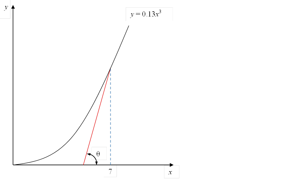
Hence
\[\tan\theta = 19.11 \nonumber\]
where
\[\theta = \text{angle made by the tangent line to the}\ x \text{-axis.} \nonumber\]
Hence
\[\begin{split} \theta &= \tan^{- 1}(19.11)\\ &= \ 87.004{^\circ} \text{ or } 1.5185 \text{ radians}\end{split} \nonumber\]
e) The equation of a straight line is
\[y = mx + c \nonumber\]
Since we know the slope of the tangent line, that is, \(19.11\), and we know one of the points on the tangent line is \((7,f(7)) = (7,0.13 \times 7^{3}) = (7,44.59)\), we can find the intercept of the straight line
\[44.59 = 19.11(7) + c \nonumber\]
\[c = - 89.18 \nonumber\]
Hence the equation of the tangent line is
\[y = 19.11x - 89.18 \nonumber\]
The tangent line crosses the \(x\)-axis when \(y=0\), that is,
\[0 = 19.11x - 89.18 \nonumber\]
\[\begin{split} x &= \frac{89.18}{19.11}\\ &= 4.667\end{split} \nonumber\]
Audiovisual Lectures
Title: Background of Newton-Raphson Method.
Summary: Learn the background Newton Raphson method of solving a nonlinear equation of the form \(f(x) = 0\). This includes finding the slope of the tangent line to the function at a particular point, finding the angle the tangent line makes to the \(x\)-axis, and finding where the tangent line to the function crosses the \(x\)-axis.
Lesson 2: Graphical Derivation of Newton-Raphson Method
Learning Objectives
After successful completion of this lesson, you should be able to
1) derive the Newton-Raphson method to solve a nonlinear equation
2) write the algorithm for the Newton-Raphson method to solve a nonlinear equation
Introduction
Methods such as the bisection method and the false position method of finding roots of a nonlinear equation \(f(x) = 0\) require bracketing of the root by two guesses. Such methods are called bracketing methods. These methods are always convergent since they are based on reducing the interval between the two guesses so as to zero in on the root of the equation.
In the Newton-Raphson method, the root is not bracketed. In fact, only one initial guess of the root is needed to get the iterative process started to find the root of an equation. The method hence falls in the category of open methods. Convergence in open methods is not guaranteed, but it does so much faster than the bracketing methods if the method does converge.
Derivation
The Newton-Raphson method is based on the principle that if the initial guess of the root of \(f(x) = 0\) is at \(x_{i}\), then if one draws the tangent to the curve at \((x_i,f(x_{i})\), the point \(x_{i + 1}\) where the tangent crosses the \(x\) -axis is an improved estimate of the root (Figure \(\PageIndex{2.1}\)). One can then use \(x_{i+1}\)as the next point to draw the tangent line to the function \(f(x)\) and find out where that tangent line crosses the \(x\) -axis. Continuing this process brings us closer and closer to the root of the equation.
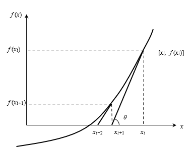
Using the definition of the slope of a function, at \(x = x_{i}\)
\[\begin{split} f^{\prime}\left( x_{i} \right)\ &= \ \tan\theta\\ &= \ \frac{f\left( x_{i} \right) - 0}{x_{i} - x_{i + 1}},\end{split} \nonumber\]
which gives
\[x_{i + 1}\ = \ x_{i} - \frac{f\left( x_{i} \right)}{f^{\prime}\left( x_{i} \right)}\;\;\;\;\;\;\;\;\;\;\;\; (\PageIndex{2.1}) \nonumber\]
Equation \((\PageIndex{2.1})\) is called the Newton-Raphson formula for solving nonlinear equations of the form \(f\left( x \right) = 0\). So starting with an initial guess, \(x_{i}\), one can find the next guess, \(x_{i + 1}\), by using Equation \((\PageIndex{2.1})\). One can repeat this process until one finds the root within a desirable tolerance.
Algorithm
The steps of the Newton-Raphson method to find the root of an equation \(f\left( x \right) = 0\) are
- Evaluate \(f^{\prime}\left( x \right)\) symbolically
- Use an initial guess of the root, \(x_{i}\), to estimate the new value of the root, \(x_{i + 1}\), as
\[x_{i + 1}\ = \ x_{i} - \frac{f\left( x_{i} \right)}{f^{\prime}\left( x_{i} \right)} \nonumber\]
- Find the absolute relative approximate error \(\left| \epsilon_{a} \right|\) as
\[\left| \epsilon_{a} \right|\ = \ \left| \frac{x_{i + 1} - \ x_{i}}{x_{i + 1}} \right| \times 100\;\;\;\;\;\;\;\;\;\;\;\; (\PageIndex{2.2}) \nonumber\]
- Compare the absolute relative approximate error with the pre-specified relative error tolerance, \(\epsilon_{s}\). If \(\left| \epsilon_{a} \right| > \epsilon_{s}\), then go to Step 2, else stop the algorithm. Also, check if the number of iterations has exceeded the maximum number of iterations allowed. If so, one needs to terminate the algorithm and notify the user.
Audiovisual Lectures
Title: Derivation of Newton-Raphson Method
Summary: Learn how to derive the Newton Raphson method of solving a nonlinear equation of the form \(f(x) = 0\).
Lesson 3: Derivation of Newton-Raphson Method from Taylor Series
Learning Objectives
After successful completion of this lesson, you should be able to
1) derive the Newton-Raphson method from the Taylor series
Introduction
The Newton-Raphson method can also be derived from the Taylor series. For a general function \(f\left( x \right)\), the Taylor series around the point \(x_{i}\) is
\[f\left( x_{i + 1} \right) = f\left( x_{i} \right) + f^{\prime}\left( x_{i} \right)\left( x_{i + 1} - x_{i} \right)+ \frac{f^{\prime\prime}\left( x_{i} \right)}{2!}\left( x_{i + 1} - x_{i} \right)^{2} + \ldots \nonumber\]
We are seeking a point where \(f\left( x \right) = 0\); that is, if we assume
\[f\left( x_{i + 1} \right) = 0, \nonumber\]
\[0 = f\left( x_{i} \right) + f^{\prime}\left( x_{i} \right)\left( x_{i + 1} - x_{i} \right) + \frac{f^{\prime\prime}\left( x_{i} \right)}{2!}\left( x_{i + 1} - x_{i} \right)^{2} + \ \ldots \nonumber\]
Using only the first two terms of the series gives
\[0 \approx f\left( x_{i} \right) + f^{\prime}\left( x_{i} \right)\left( x_{i + 1} - x_{i} \right) \nonumber\]
Solving for \(x_{i + 1}\) gives
\[x_{i + 1} \approx x_{i} - \frac{f\left( x_{i} \right)}{f^{\prime}\left( x_{i} \right)} \nonumber\]
This is the same Newton-Raphson method formula as derived in the previous lesson using geometry and differential calculus.
Audiovisual Lectures
Title: Newton-Raphson Method Derivation from Taylor Series
Summary: This video discusses how to derive Newton Raphson method from Taylor's theorem.
Lesson 4: Application of Newton-Raphson Method
Learning Objectives
After successful completion of this lesson, you should be able to
1) apply the Newton-Raphson method to solve for roots of a nonlinear equation.
Applications
In the previous lessons, we discussed the background to the Newton-Raphson Method of solving nonlinear equations. In this lesson, we take an example of how to apply the algorithm of the Newton-Raphson method to solve a nonlinear equation.
Solve the nonlinear equation \(x^{3} = 20\) by the Newton-Raphson method using an initial guess of \(x_{0} = 3\).
Conduct three iterations to estimate the root of the above equation.
Find the absolute relative approximate error at the end of each iteration.
Find the number of significant digits at least correct at the end of each iteration.
Solution
First, we rewrite the equation \(x^{3} = 20\) in the form \(f(x) = 0\)
\[f(x) = x^{3} - 20 \nonumber\]
\[f^{\prime}(x) = 3x^{2} \nonumber\]
The initial guess is
\[x_{0} = 3 \nonumber\]
Iteration 1
The estimate of the root is
\[\begin{split} x_{1} &= x_{0} - \frac{f(x_{0})}{f^{\prime}(x_{0})}\\ &= 3 - \frac{3^{3} - 20}{(3)^{2}}\\ &= 3 - \frac{7}{27}\\ &= 3 - 0.259259\\ &= 2.74074\end{split} \nonumber\]
The absolute approximate relative error \(\left| \epsilon_{a} \right|\) at the end of Iteration 1 is
\[\begin{split} \left| \epsilon_{a} \right| &= \left| \frac{x_{1} - x_{o}}{x_{1}} \right| \times 100\\ &= \left| \frac{2.74074 - 3}{2.74074} \right| \times 100\\ &= 9.46\%\end{split} \nonumber\]
The number of significant digits at least correct is \(0\), as you need an absolute relative approximate error of \(5 \%\) or less for at least one significant digit to be correct in your result.
Iteration 2
The estimate of the root is
\[\begin{split} x_{2} &= x_{1} - \frac{f(x_{1})}{f^{\prime}(x_{1})}\\ &= 2.74074 - \frac{(2.74074)^{3} - 20}{3(2.74074)^{2}}\\ &= 2.74074 - \frac{0.587495}{22.5350}\\ &= 2.71467 \end{split} \nonumber\]
The absolute relative approximate error \(\left| \epsilon_{a} \right|\) at the end of Iteration 2 is
\[\begin{split} \left| \epsilon_{a} \right| &= \left| \frac{x_{2} - x_{1}}{x_{2}} \right| \times 100\\ &= \left| \frac{2.71467 - 2.74074}{2.71467} \right| \times 100\\ &= 0.960\% \end{split} \nonumber\]
The maximum value of \(m\) for which \(\left| \epsilon_{a} \right|\leq0.5 \times 10^{2 - m}\%\) is \(1.71669\). Hence, the number of significant digits at least correct is \(1\).
Iteration 3
The estimate of the root is
\[\begin{split} x_{3} &= x_{2} - \frac{f(x_{2})}{f^{\prime}(x_{2})}\\ &= 2.71467 - \frac{(2.71467)^{3} - 20}{(2.71476)^{2}}\\ &= 2.71467 - \frac{5.57925 \times 10^{- 3}}{22.1083}\\ &= 2.71467 - 2.52360 \times 10^{- 4}\\ &= 2.71442\end{split} \nonumber\]
The absolute relative approximate error \(\left| \epsilon_{a} \right|\)at the end of Iteration 3 is
\[\begin{split} \left| \epsilon_{a} \right| &= \left| \frac{2.71442 - 2.71467}{2.71442} \right| \times 100\\ &= 0.00921\% \end{split} \nonumber\]
The maximum value of \(m\) for which\(\ \left| \epsilon_{a} \right|\leq 0.5 \times 10^{2 - m}\%\) is\(\ 3.73471\). Hence, the number of significant digits at least correct is \(3\).
You are working for ‘DOWN THE TOILET COMPANY’ that makes floats for ABC commodes. The floating ball has a specific gravity of \(0.6\) and has a radius of \(5.5\ \text{cm}\). You are asked to find the depth to which the ball is submerged when floating in the water.
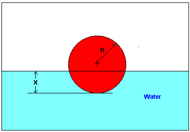
The equation that gives the depth \(x\) in meters to which the ball is submerged underwater is given by
\[x^{3} - 0.165x^{2} + 3.993 \times 10^{- 4} = 0 \nonumber\]
Use the Newton-Raphson method of finding roots of equations to find
a) the depth \(x\) to which the ball is submerged underwater. Conduct three iterations to estimate the root of the above equation.
b) the absolute relative approximate error at the end of each iteration, and
c) the number of significant digits at least correct at the end of each iteration.
Solution
\[f\left( x \right) = x^{3} - 0.165x^{2} + 3.993 \times 10^{- 4} \nonumber\]
\[f^{\prime}\left( x \right) = 3x^{2} - 0.33x \nonumber\]
Let us assume the initial guess of the root of \(f\left( x \right) = 0\) is \(x_{0} = 0.05\text{ m}.\) This is a reasonable guess (discuss why \(x = 0\) and \(x = 0.11\text{ m}\) are not good choices) as the extreme values of the depth \(x\) would be \(0\) and the diameter (\(0.11\ \text{m}\)) of the ball.
Iteration 1
The estimate of the root is
\[\begin{split} x_{1} &= x_{0} - \frac{f\left( x_{0} \right)}{f^{\prime}\left( x_{0} \right)}\\ &= 0.05 - \frac{\left( 0.05 \right)^{3} - 0.165\left( 0.05 \right)^{2} + 3.993 \times 10^{- 4}}{3\left( 0.05 \right)^{2} - 0.33\left( 0.05 \right)}\\ &= 0.05 - \frac{1.118 \times 10^{- 4}}{- 9 \times 10^{- 3}}\\ &= 0.05 - \left( - 0.01242 \right)\\ &= 0.06242 \end{split} \nonumber\]
The absolute relative approximate error \(\left| \epsilon_{a} \right|\) at the end of Iteration 1 is
\[\begin{split} \left| \epsilon_{a} \right| &= \left| \frac{x_{1} - x_{0}}{x_{1}} \right| \times 100\\ &= \left| \frac{0.06242 - 0.05}{0.06242} \right| \times 100\\ &=19.90\% \end{split} \nonumber\]
The number of significant digits at least correct is \(0\), as you need an absolute relative approximate error of \(5\%\) or less for at least one significant digit to be correct in your result.
Iteration 2
The estimate of the root is
\[\begin{split} x_{2} &= x_{1} - \frac{f\left( x_{1} \right)}{f^{\prime}\left( x_{1} \right)}\\ &= 0.06242 - \frac{\left( 0.06242 \right)^{3} - 0.165\left( 0.06242 \right)^{2} + 3.993 \times 10^{- 4}}{3\left( 0.06242 \right)^{2} - 0.33\left( 0.06242 \right)}\\ &= 0.06242 - \frac{- 3.97781 \times 10^{- 7}}{- 8.90973 \times 10^{- 3}}\\ &= 0.06242 - \left( 4.4646 \times 10^{- 5} \right)\\ &= 0.06238 \end{split} \nonumber\]
The absolute relative approximate error \(\left| \epsilon_{a} \right|\) at the end of Iteration 2 is
\[\begin{split} \left| \epsilon_{a} \right| &= \left| \frac{x_{2} - x_{1}}{x_{2}} \right| \times 100\\ &= \left| \frac{0.06238 - 0.06242}{0.06238} \right| \times 100\\ &= 0.0716\% \end{split} \nonumber\]
The maximum value of \(m\) for which \(\left| \epsilon_{a} \right| \leq 0.5 \times 10^{2 - m}\) is \(2.844\). Hence, the number of significant digits at least correct in the answer is \(2\).
Iteration 3
The estimate of the root is
\[\begin{split} x_{3} &= x_{2} - \frac{f\left( x_{2} \right)}{f^{\prime}\left( x_{2} \right)}\\ &= 0.06238 - \frac{\left( 0.06238 \right)^{3} - 0.165\left( 0.06238 \right)^{2} + 3.993 \times 10^{- 4}}{3\left( 0.06238 \right)^{2} - 0.33\left( 0.06238 \right)}\\ &= 0.06238 - \frac{4.44 \times 10^{- 11}}{- 8.91171 \times 10^{- 3}}\\ &= 0.06238 - \left( - 4.9822 \times 10^{- 9} \right)\\ &= 0.06238 \end{split} \nonumber\]
The absolute relative approximate error \(\left| \epsilon_{a} \right|\) at the end of Iteration 3 is
\[\begin{split} \left| \epsilon_{a} \right| &= \left| \frac{0.06238 - 0.06238}{0.06238} \right| \times 100\\ &= 0 \end{split} \nonumber\]
The number of significant digits at least correct is \(4\), as only \(4\) significant digits are carried through in all the calculations.
Lesson 5: Advantages and Pitfalls of the Newton-Raphson Method
Learning Objectives
After successful completion of this lesson, you should be able to
1) enumerate the advantages of the Newton-Raphson method and the reasoning behind them.
2) list the drawbacks of the Newton-Raphson method and the reason behind them.
Advantages of the Newton-Raphson Method
1) Fast convergence: Newton-Raphson method converges fast when it converges. The method converges quadratically – one can interpret that the number of significant digits correct gets approximately squared at each iteration.
2) Only one initial estimate is needed: Newton-Raphson method is an open method that requires only one initial estimate of the root of the equation. However, since the method is an open method, convergence is not guaranteed.
Drawbacks of the Newton-Raphson Method
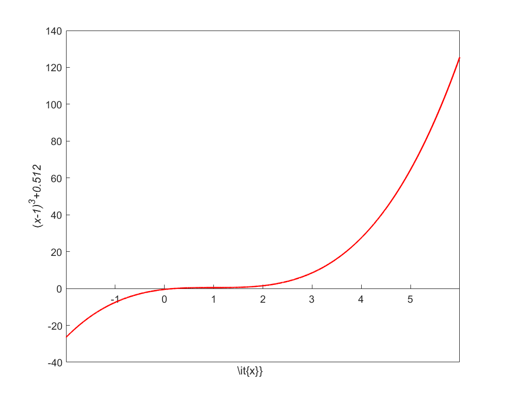
1) Divergence at inflection points: If the selection of the initial guess or an iterated value of the root turns out to be close to the inflection point of the function \(f\left( x \right)\) in the equation \(f\left( x \right) = 0\), Newton-Raphson method may start diverging away from the root. It may then begin to converging back to the root. For example, to find the root of the equation
\[f\left( x \right) = \left( x - 1 \right)^{3} + 0.512 = 0 \nonumber\]
then
\[f^\prime(x) = 3(x-1)^2 \nonumber\]
and the Newton-Raphson method reduces to
\[x_{i + 1}\ = \ x_{i} - \frac{({x_{i}}^{3} - 1)^{3} + 0.512}{3(x_{i} - 1)^{2}} \nonumber\]
Starting with an initial guess of \(x_{0} = 5.0\), Table \(\PageIndex{5.1}\) shows the iterated values of the root of the equation. As you can observe, the root starts to diverge at Iteration 6 because the previous estimate of \(0.92589\) is close to the inflection point of \(x = 1\) (the value of \(f^\prime\left( x \right)\) is zero at the inflection point). Eventually, after \(12\) more iterations, the root converges to the exact value of \(x = 0.2\).
| \(\text{Iteration Number}\) | \(x_{i}\) |
|---|---|
| \(0\) | \(5.0000\) |
| \(1\) | \(3.6560\) |
| \(2\) | \(2.7465\) |
| \(3\) | \(2.1084\) |
| \(4\) | \(1.6000\) |
| \(5\) | \(0.92589\) |
| \(6\) | \(-30.119\) |
| \(7\) | \(-19.746\) |
| \(8\) | \(-12.831\) |
| \(9\) | \(-8.2217\) |
| \(10\) | \(-5.1498\) |
| \(11\) | \(-3.1044\) |
| \(12\) | \(-1.7464\) |
| \(13\) | \(-0.85356\) |
| \(14\) | \(-0.28538\) |
| \(15\) | \(0.039784\) |
| \(16\) | \(0.17475\) |
| \(17\) | \(0.19924\) |
| \(18\) | \(0.2\) |
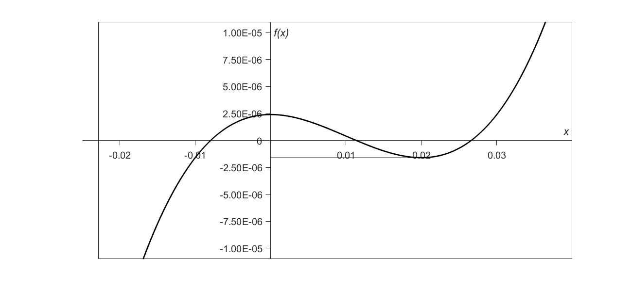
2) Division by zero: Division by zero may occur during the implementation of the Newton-Raphson method. For example, for the equation
\[f(x) = x^{3} - 0.03 x^{2} + 2.4 \times 10^{-6} = 0 \nonumber\]
we have
\[f^\prime(x) = 3x^2-0.06x \nonumber\]
and the Newton-Raphson method reduces to
\[x_{i + 1}\ = \ x_{i} - \frac{x_{i}^{3} - 0.03x_{i}^{2} + 2.4 \times 10^{- 6}}{3x_{i}^{2} - 0.06x_{i}} \nonumber\]
For \(x_{0} = 0\) or \(x_{0} = 0.02\), division by zero occurs (Figure \(\PageIndex{5.2}\)). For an initial guess close to \(0.02\), such as \(x_{0} = 0.01999\), one may avoid division by zero, but then the denominator in the formula is a small number. For this case of initial guess of \(x_{0}=0.01999\), as given in Table \(\PageIndex{5.2}\), even after 9 iterations, the Newton-Raphson method does not converge.
| \(\text{Iteration Number}\) | \(x_{i}\) | \(f(x_{i})\) | \(\left| \in_{a} \right|\%\) |
|---|---|---|---|
| \(0\) | \(0.019990\) | \(-1.6000 \times 10^{-6}\) | \(---\) |
| \(1\) | \(-2.6480\) | \(18.778\) | \(100.75\) |
| \(2\) | \(-1.7620\) | \(-5.5638\) | \(50.282\) |
| \(3\) | \(-1.1714\) | \(-1.6485\) | \(50.422\) |
| \(4\) | \(-0.77765\) | \(-0.48842\) | \(50.632\) |
| \(5\) | \(-0.51518\) | \(-0.14470\) | \(50.946\) |
| \(6\) | \(-0.34025\) | \(-0.042862\) | \(51.413\) |
| \(7\) | \(-0.22369\) | \(-0.012692\) | \(52.107\) |
| \(8\) | \(-0.14608\) | \(-0.0037553\) | \(53.127\) |
| \(9\) | \(-0.094490\) | \(-0.0011091\) | \(54.602\) |
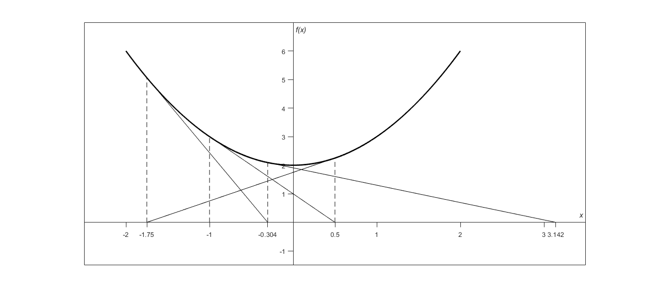
3) Oscillations near local maximum and minimum: Results obtained from the Newton-Raphson method may oscillate about the local maximum or minimum without converging on a root but converging on the local maximum or minimum. Eventually, it may lead to division by a number close to zero and may diverge.
For example, for
\[f\left( x \right) = x^{2} + 2 = 0 \nonumber\]
the equation has no real roots (Figure \(\PageIndex{5.3}\) and Table \(\PageIndex{5.3}\)).
| \(\text{Iteration Number}\) | \(x_{i}\) | \(f(x_{i})\) | \(\left| \in_{a} \right|\%\) |
|---|---|---|---|
| \(0\) | \(-1.0000\) | \(3.00\) | \(---\) |
| \(1\) | \(0.5\) | \(2.25\) | \(300.00\) |
| \(2\) | \(-1.75\) | \(5.063\) | \(128.571\) |
| \(3\) | \(-0.30357\) | \(2.092\) | \(476.47\) |
| \(4\) | \(3.1423\) | \(11.874\) | \(109.66\) |
| \(5\) | \(1.2529\) | \(3.570\) | \(150.80\) |
| \(6\) | \(-0.17166\) | \(2.029\) | \(829.88\) |
| \(7\) | \(5.7395\) | \(34.942\) | \(102.99\) |
| \(8\) | \(2.6955\) | \(9.266\) | \(112.93\) |
| \(9\) | \(0.97678\) | \(2.954\) | \(175.96\) |
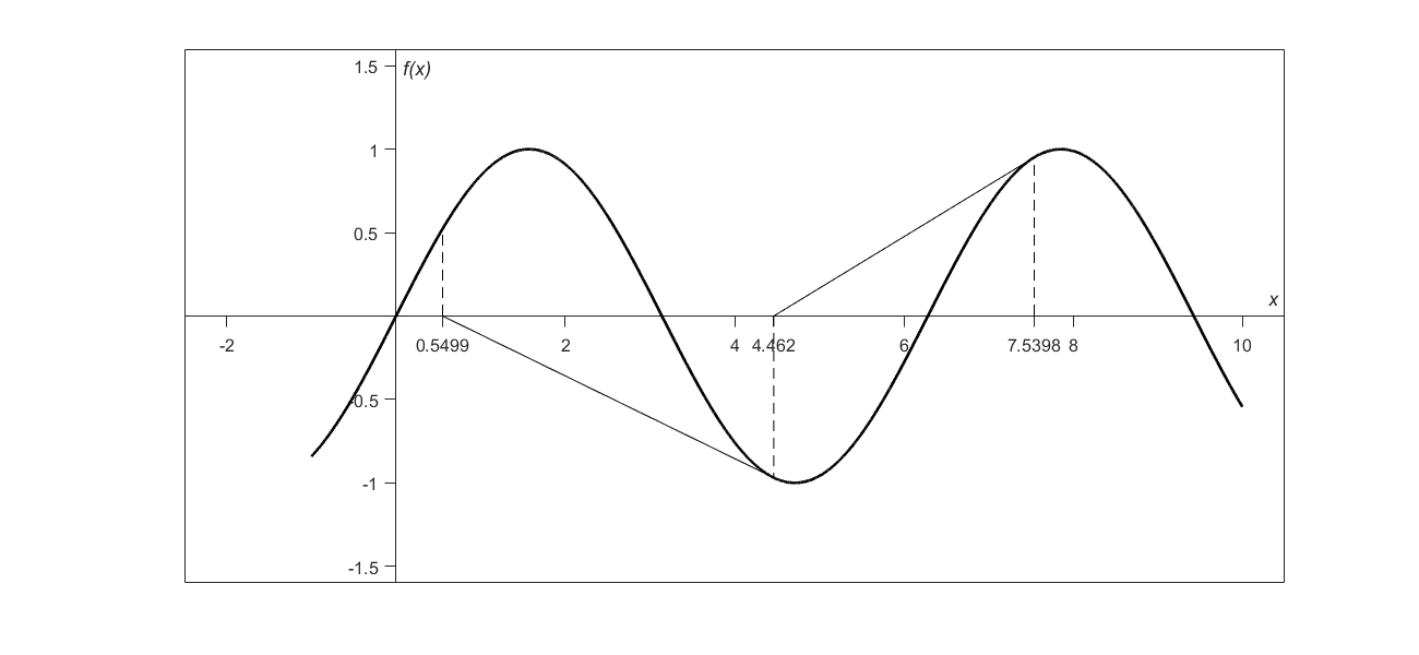
4) Root jumping: In some cases where the function \(f(x)\) is oscillating and has several roots, one may choose an initial guess close to a root. However, the guesses may jump and converge to some other root. For example, for solving the equation \(\sin x = 0\) if you choose \(x_{0} = 2.4\pi = \left( 7.539822 \right)\) as an initial guess, it converges to the root of \(x = 0,\) as shown in Table 4 and Figure 4. However, one may have chosen this as an initial guess to converge to \(x = 2\pi = 6.2831853\).
| \(\text{Iteration Number}\) | \(x_{i}\) | \(f(x_{i})\) | \(\left| \in_{a} \right|\%\) |
|---|---|---|---|
| \(0\) | \(7.539822\) | \(0.951\) | \(---\) |
| \(1\) | \(4.462\) | \(-0.969\) | \(68.973\) |
| \(2\) | \(0.5499\) | \(0.5226\) | \(711.44\) |
| \(3\) | \(-0.06307\) | \(-0.06303\) | \(971.91\) |
| \(4\) | \(8.376 \times 10^{- 4}\) | \(8.375 \times 10^{- 5}\) | \(7.54 \times 10^{4}\) |
| \(5\) | \(-1.95861 \times 10^{- 13}\) | \(-1.95861 \times 10^{- 13}\) | \(4.28 \times 10^{10}\) |
Audiovisual Lectures
Title: Newton-Raphson Method: Advantages and Drawbacks
Summary: This video discusses the advantages and drawbacks of Newton Raphson method of solving nonlinear equations.
Part 1
Part 2
Appendix A. What is an inflection point?
For a function \(f\left( x \right)\), the point where the concavity changes from up-to-down or down-to-up is called its inflection point; that is, the sign of curvature changes sign. For example, for the function \(f\left( x \right) = \left( x - 1 \right)^{3}\), the concavity changes at \(x = 1\), and hence (1,0) is an inflection point.
For a function \(f\left( x \right)\), for \((x,f\left( x \right))\) to be an inflection point, \(f^{\prime\prime}(x) = 0\) is a necessary condition. However, an inflection point may or may not exist at a point where \(f^{\prime\prime}(x) = 0\). For example, for \(f(x) = x^{4} - 16\), \(f^{\prime\prime}(0) = 0\), but the concavity does not change at \(x = 0\). Hence the point \((0, -16)\) is not an inflection point of \(f(x) = x^{4} - 16\).
For \(f\left( x \right) = \left( x - 1 \right)^{3}\), \(f^{\prime\prime}(1) = 0\) and \(f^{\prime\prime}(x)\) changes sign at \(x = 1\) (\(f^{\prime\prime}(x) < 0\) for \(x = 1^{-}\), and \(f^{\prime\prime}(x) > 0\) for \(x = 1^{+}\)), and thus brings up the Inflection Point Theorem for a function \(f(x)\), which states the following.
“If \(f^\prime(c)\) exists and \(f^{\prime\prime}(c)\) changes sign at \(x = c\), then the point \((c,f(c))\) is an inflection point of the graph of \(f\).”
Multiple Choice Test
(1). The Newton-Raphson method of finding roots of nonlinear equations falls under the category of _____________ methods.
(A) bracketing
(B) open
(C) random
(D) graphical
(2). The Newton-Raphson method formula for finding the square root of a real number \(R\) from the equation \(x^{2} - R = 0\) is,
(A) \(\displaystyle x_{i + 1} = \frac{x_{i}}{2}\)
(B) \(\displaystyle x_{i + 1} = \frac{3x_{i}}{2}\)
(C) \(\displaystyle x_{i + 1} = \frac{1}{2}\left( x_{i} + \frac{R}{x_{i}} \right)\)
(D) \(\displaystyle x_{i + 1} = \frac{1}{2}\left( 3x_{i} - \frac{R}{x_{i}} \right)\)
(3). The next iterative value of the root of \(x^{2}-4=0\) using the Newton-Raphson method, if the initial guess is \(3\), is
(A) \(1.5\)
(B) \(2.067\)
(C) \(2.167\)
(D) \(3.000\)
(4). The root of the equation \(f(x) = 0\) is found by using the Newton-Raphson method. The initial estimate of the root is \(x_{0} = 3\), \(f\left( 3 \right) = 5\). The angle made by the line tangent to the function \(f(x)\) makes at \(x = 3\) is \(57{^\circ}\) with respect to the \(x\)-axis. The next estimate of the root, \(x_{1}\) most nearly is
(A) \(-3.2470\)
(B) \(-0.24704\)
(C) \(3.2470\)
(D) \(6.2470\)
(5). The root of \(x^{3} = 4\) is found by using the Newton-Raphson method. The successive iterative values of the root are given in the table below.
| Iteration Number | Value of Root |
|---|---|
| \(0\) | \(2.0000\) |
| \(1\) | \(1.6667\) |
| \(2\) | \(1.5911\) |
| \(3\) | \(1.5874\) |
| \(4\) | \(1.5874\) |
The iteration number at which I would first trust at least two significant digits in the answer is
(A) \(1\)
(B) \(2\)
(C) \(3\)
(D) \(4\)
(6). The ideal gas law is given by
\(pv = RT\)
where \(p\) is the pressure, \(v\) is the specific volume, \(R\) is the universal gas constant, and \(T\) is the absolute temperature. This equation is only accurate for a limited range of pressure and temperature. Vander Waals came up with an equation that was accurate for a larger range of pressure and temperature, given by
\[ \left( p + \frac{a}{v^{2}} \right)\left( v - b \right) = RT \nonumber\]
where a and b are empirical constants dependent on a particular gas. Given the value of \(R = 0.08\), \(a = 3.592\), \(b = 0.04267\), \(p = 10\) and \(T = 300\) (assume all units are consistent), one is going to find the specific volume, \(v\), for the above values. Without finding the solution from the Vander Waals equation, what would be a good initial guess for \(v\)?
(A) \(0\)
(B) \(1.2\)
(C) \(2.4\)
(D) \(3.6\)
For complete solution, go to
http://nm.mathforcollege.com/mcquizzes/03nle/quiz_03nle_newton_solution.pdf
Problem Set
(1). Find the estimate of the root of \(x^{2} - 4 = 0\) by using the Newton-Raphson method. Assume that the initial guess of the root is \(3\). Conduct three iterations. Also, calculate the approximate error, true error, absolute relative approximate error, and absolute relative true error at the end of each iteration.
- Answer
-
Iteration # Root Estimate Approx Error True Error Abs Rel Appr Err Abs Rel True Err \(1\) \(2.1667\) \(0.8333\) \(-0.1667\) \(27.77\%\) \(8.335\%\) \(2\) \(2.0064\) \(-0.1603\) \(-0.0064\) \(7.98\%\) \(0.32\%\) \(3\) \(2.0002\) \(-0.0062\) \(-0.0002\) \(0.31\%\) \(0.001\%\)
(2). The velocity of a body is given by \(v(t) = 5e^{- t} + 6\), where \(v\) is in m/s and \(t\) is in seconds.
a) Use the Newton Raphson method to find the time when the velocity will be \(7.0\) m/s. Use two iterations and take \(t = 2\) seconds as the initial guess.
b) What is the relative true error at the end of the second iteration for part (a)?
- Answer
-
\(a)\ 1.5236,\ 1.6058\ \ b) \ 0.2260\%\)
(3). You are working for DOWN THE TOILET COMPANY that makes floats for ABC commodes. The ball has a specific gravity of \(0.6\) and has a radius of \(5.5\) cm. You are asked to find the depth to which the ball will get submerged when floating in the water.

The equation that gives the depth \(x\) (unit of \(x\) is meters) to which the ball is submerged under water is given by
\[x^{3} - 0.165x^{2} + 3.993 \times 10^{- 4} = 0 \nonumber\]
Solving it exactly would require some effort. However, using numerical techniques such as Newton-Raphson method, we can solve this equation and any other equation of the form \(f(x) = 0\). Solve the above equation by the Newton-Raphson method and do the following.
a) Conduct three iterations. Use an initial guess \(x = 0.055\ \text{m}\).
b) Calculate the absolute relative approximate error at the end of each step.
c) Find the number of significant digits at least correct at the end of each iteration.
d) How could you have used the knowledge of the physics of the problem to develop initial guess for the Newton-Raphson method?
- Answer
-
\(a)\ 0.06233,\ 0.06237,\ 0.06237\)
\(b)\ n/a,\ 0.06413\%,\ 0\%\)(\(0\%\) if only 4 significant digits were carried in the calculations)
\(c)\ 0,\ 2,\ 4\) (as only 4 significant digits were carried in the calculations)
\(d)\) Since the diameter is \(0.11\ \text{m}\), a value of \(0\) or \(0.11\) seems to be a good initial estimate, but these guesses give division by zero. So, \(0.055\) would be a good initial estimate.
(4). The root of the equation \(f(x) = 0\) is found by using the Newton-Raphson method. If the initial estimate of the root is assumed to be \(x_{0} = 3\), given \(f(3) = 5\), and the angle the tangent makes to the function \(f(x)\) at \(x = 3\) is \(57^{\circ}\), what is the next estimate of the root, \(x_{1}\)?
- Answer
-
\(-0.24696\)
(5). The root of the equation \(f(x) = 0\) is found by using the Newton-Raphson method. The initial estimate of the root is assumed to be \(x_{0} = 5.0\), and the angle the tangent makes with the \(x\)-axis to the function \(f(x)\) at \(x_{0} = 5.0\) is \(89.236^{\circ}\). If the next estimate of the root is, \(x_{1} = 3.693\), what is the value of the function \(f(x)\) at \(x = 5\)?
- Answer
-
\(98.012\)
(6). Find the Newton-Raphson method formula for finding the square root of a real number \(R\) from the equation \(x^{2} - R = 0\). Find the square root of \(50.41\) by using the formula. Assume \(50.41\) as the initial guess. How many iterations does it take to get at least \(3\) significant digits correct in your answer? Do not use the true value to answer the question.
- Answer
-
Takes 6 iterations. Root at the end of 6th iteration is \(7.100\), with the absolute relative approx error of \(0.014\%\). Four significant digits were used in solving the problem.


