4.2.1: Case n=3

The Euler-Poisson-Darboux equation in this case is

$$(rM)_{rr}=c^{-2}(rM)_{tt}.\]

Thus $rM$ is the solution of the one-dimensional wave equation with initial data

$$\begin{equation} \label{initialn3}\tag{4.2.1.1} (rM)(r,0)=rF(r)\ \ \ (rM)_t(r,0)=rG(r). \end{equation}$$
From the d'Alembert formula we get formally
$$\begin{eqnarray} \label{meansol1} M(r,t)&=&\dfrac{(r+ct)F(r+ct)+(r-ct)F(r-ct)}{2r}\\ \tag{4.2.1.2} &&+\dfrac{1}{2cr}\int_{r-ct}^{r+ct}\ \xi G(\xi)\ d\xi. \end{eqnarray}$$

The right hand side of the previous formula is well defined if the domain of dependence $[x-ct,x+ct]$ is a subset of $(0,\infty)$. We can extend $F$ and $G$ to $F_0$ and $G_0$ which are defined on $(-\infty,\infty)$ such that $rF_0$ and $rG_0$ are $C^2(\mathbb{R}^1)$-functions as follows.
Set

$$
F_0(r)=\left\{ $$\begin{array}{r@{\quad:\quad}l} F(r)&r>0\\ f(x)&r=0\\ F(-r)&r<0 \end{array}$$ \right.\
\]

The function $G_0(r)$ is given by the same definition where $F$ and $f$ are replaced by $G$ and $g$, respectively.

Lemma. $rF_0(r),\ rG_0(r)\in C^2(\mathbb{R}^2)$.

Proof. From definition of $F(r)$ and $G(r)$, $r>0$, it follows from the mean value theorem

$$\lim_{r\to+0} F(r)=f(x),\ \ \ \lim_{r\to+0} G(r)=g(x).\]

Thus $rF_0(r)$ and $rG_0(r)$ are $C(\mathbb{R}^1)$-functions. These functions are also in $C^1(\mathbb{R}^1)$. This follows since $F_0$ and $G_0$ are in $C^1(\mathbb{R}^1)$. We have, for example,

$$\begin{eqnarray*} F'(r)&=&\dfrac{1}{\omega_n}\int_{\partial B_1(0)}\ \sum_{j=1}^n f_{y_j}(x+r\xi)\xi_j\ dS_\xi\\ F'(+0)&=&\dfrac{1}{\omega_n}\int_{\partial B_1(0)}\ \sum_{j=1}^n f_{y_j}(x)\xi_j\ dS_\xi\\ &=&\dfrac{1}{\omega_n}\sum_{j=1}^n f_{y_j}(x)\int_{\partial B_1(0)}\ n_j\ dS_\xi\\ &=&0. \end{eqnarray*}$$

Then, $rF_0(r)$ and $rG_0(r)$ are in $C^2(\mathbb{R}^1)$, provided $F''$ and $G''$ are bounded as $r\to+0$. This property follows from

$$F''(r)=\dfrac{1}{\omega_n}\int_{\partial B_1(0)}\ \sum_{i,j=1}^n f_{y_iy_j}(x+r\xi)\xi_i\xi_j\ dS_\xi.\]

Thus

$$F''(+0)=\dfrac{1}{\omega_n}\sum_{i,j=1}^n f_{y_iy_j}(x)\int_{\partial B_1(0)}\ n_in_j\ dS_\xi.\]

We recall that $f,g\in C^2(\mathbb{R}^2)$ by assumption.

$\Box$

The solution of the above initial value problem, where $F$ and $G$ are replaced by $F_0$ and $G_0$, respectively, is

$$\begin{eqnarray*} M_0(r,t)&=&\dfrac{(r+ct)F_0(r+ct)+(r-ct)F_0(r-ct)}{2r}\\ &&+\dfrac{1}{2cr}\int_{r-ct}^{r+ct}\ \xi G_0(\xi)\ d\xi. \end{eqnarray*}$$

Since $F_0$ and $G_0$ are even functions, we have

$$\int_{r-ct}^{ct-r}\ \xi G_0(\xi)\ d\xi=0.\]

Thus

$$\begin{eqnarray} M_0(r,t)&=&\dfrac{(r+ct)F_0(r+ct)-(ct-r)F_0(ct-r)}{2r}\nonumber\\ \label{meansol2} \tag{4.2.1.3} &&+\dfrac{1}{2cr}\int_{ct-r}^{ct+r}\ \xi G_0(\xi)\ d\xi, \end{eqnarray}$$

see Figure 4.2.1.1.

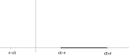
Figure 4.2.1.1: Changed domain of integration

For fixed $t>0$ and $0<r<ct$ it follows that $M_0(r,t)$ is the solution of the initial value problem with given initially data ($\ref{initialn3}$) since $F_0(s)=F(s)$, $G_0(s)=G(s)$ if $s>0$.

Since for fixed $t>0$

$$u(x,t)=\lim_{r\to 0} M_0(r,t),\]

it follows from d'Hospital's rule that

$$\begin{eqnarray*} u(x,t)&=&ctF'(ct)+F(ct)+tG(ct)\\ &=&\dfrac{d}{dt}\left(tF(ct)\right)+tG(ct). \end{eqnarray*}$$

Theorem 4.2. Assume $f\in C^3(\mathbb{R}^3)$ and $g\in C^2(\mathbb{R}^3)$ are given. Then there exists a unique solution $u\in C^2(\mathbb{R}^3\times [0,\infty))$ of the initial value problem (4.2.2)-(4.2.3), where $n=3$, and the solution is given by the Poisson's formula

$$\begin{eqnarray} u(x,t)&=&\dfrac{1}{4\pi c^2}\dfrac{\partial}{\partial t}\left(\dfrac{1}{t}\int_{\partial B_{ct}(x)}\ f(y)\ dS_y\right)\\ \tag{4.2.1.4} &&+\dfrac{1}{4\pi c^2 t}\int_{\partial B_{ct}(x)}\ g(y)\ dS_y. \end{eqnarray}$$

Proof. Above we have shown that a $C^2$-solution is given by Poisson's formula. Under the additional assumption $f\in C^3$ it follows from Poisson's formula that this formula defines a solution which is in $C^2$, see F. John [10], p. 129.

$\Box$

Corollary. From Poisson's formula we see that the domain of dependence for $u(x,t_0)$ is the intersection of the cone defined by $|y-x|=c|t-t_0|$ with the hyperplane defined by $t=0$, see Figure 4.2.1.2.

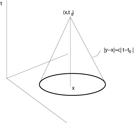
Figure 4.2.1.2: Domain of dependence, case $n=3$.

Contributors and Attributions

• Prof. Dr. Erich Miersemann (Universität Leipzig)

• Integrated by Justin Marshall.