4.4: A Method of Riemann

Riemann's method provides a formula for the solution of the following Cauchy initial value problem for a hyperbolic equation of second order in two variables. Let

$${\mathcal S}:\ \ x=x(t), y=y(t),\ \ t_1\le t \le t_2,\]

be a regular curve in $\mathbb{R}^2$, that is, we assume $x,\ y\in C^1[t_1,t_2]$ and $x'^2+y'^2\not=0$. Set

$$Lu:=u_{xy}+a(x,y)u_x+b(x,y)u_y+c(x,y)u,\]

where $a,\ b\in C^1$ and $c,\ f\in C$ in a neighborhood of ${\mathcal S}$. Consider the initial value problem

$$\begin{eqnarray} \label{riem1} Lu&=&f(x,y)\\ \label{riem2} u_0(t)&=&u(x(t),y(t))\\ \label{riem3} p_0(t)&=&u_x(x(t),y(t))\\ \label{riem4} q_0(t)&=&u_y(x(t),y(t)), \end{eqnarray}$$

where $f\in C$ in a neighbourhood of ${\mathcal S}$ and $u_0,\ p_0,\ q_0\in C^1$ are given.

We assume:

1. $u_0'(t)=p_0(t)x'(t)+q_0(t)y'(t)$ (strip condition),
2. ${\mathcal S}$ is not a characteristic curve. Moreover assume that the characteristic curves, which are lines here and are defined by $x=const.$ and $y=const.$, have at most one point of intersection with ${\mathcal S}$, and such a point is not a touching point, i. e., tangents of the characteristic and ${\mathcal S}$ are different at this point.

We recall that the characteristic equation to ($\ref{riem1}$) is $\chi_x\chi_y=0$ which is satisfied if $\chi_x(x,y)=0$ or $\chi_y(x,y)=0$. One family of characteristics associated to these first partial differential of first order is defined by $x'(t)=1,\ y'(t)=0$, see Chapter 2.

Assume $u,\ v\in C^1$ and that $u_{xy},\ v_{xy}$ exist and are continuous. Define the adjoint differential expression by

$$Mv=v_{xy}-(av)_x-(bv)_y+cv.\]

We have

$$\begin{equation} \label{riem5} 2(vLu-uMv)=(u_xv-v_xu+2buv)_y+(u_yv-v_yu+2auv)_x. \end{equation}$$

Set

$$\begin{eqnarray*} P&=&-(u_xv-x_xu+2buv)\\ Q&=&u_yv-v_yu+2auv. \end{eqnarray*}$$

From ($\ref{riem5}$) it follows for a domain $\Omega\in\mathbb{R}^2$

$$\begin{eqnarray} 2\int_\Omega\ (vLu-uMv)\ dxdy&=&\int_\Omega\ (-P_y+Q_x)\ dxdy\nonumber\\ \label{riem6} &=&\oint\ Pdx+Qdy, \end{eqnarray}$$

where integration in the line integral is anticlockwise. The previous equation follows from Gauss theorem or after integration by parts:

$$\int_\Omega\ (-P_y+Q_x)\ dxdy=\int_{\partial\Omega}\ (-Pn_2+Qn_1)\ ds,\]

where $n=(dy/ds,-dx/ds)$, $s$ arc length, $(x(s),y(s))$ represents $\partial\Omega$.

Assume $u$ is a solution of the initial value problem ($\ref{riem1}$)-($\ref{riem4}$) and suppose that $v$ satisfies

$$Mv=0\ \ \mbox{in}\ \Omega.\]

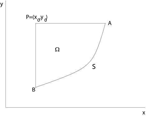
Figure 4.4.1: Riemann's method, domain of integration

Then, if we integrate over a domain $\Omega$ as shown in Figure 4.4.1, it follows from ($\ref{riem6}$) that

$$\begin{equation} \label{riem7} 2\int_\Omega\ vf\ dxdy=\int_{BA}\ Pdx+Qdy+\int_{AP}\ Pdx+Qdy+\int_{PB}\ Pdx+Qdy. \end{equation}$$

The line integral from $B$ to $A$ is known from initial data, see the definition of $P$ and $Q$.

Since

$$u_xv-v_xu+2buv=(uv)_x+2u(bv-v_x),\]

it follows

$$\begin{eqnarray*} \int_{AP} Pdx+Qdy&=&-\int_{AP} \left((uv)_x+2u(bv-v_x)\right)\ dx\\ &=&-(uv)(P)+(uv)(A)-\int_{AP}\ 2u(bv-v_x)\ dx. \end{eqnarray*}$$

By the same reasoning we obtain for the third line integral

$$\begin{eqnarray*} \int_{PB} Pdx+Qdy&=&\int_{PB} \left((uv)_y+2u(av-v_y)\right)\ dy\\ &=&(uv)(B)-(uv)(P)+\int_{PB} 2u(av-v_y)\ dy. \end{eqnarray*}$$

Combining these equations with ($\ref{riem6}$), we get

$$\begin{eqnarray} 2v(P)u(P)&=&\int_{BA} (u_xv-v_x+2buv)\ dx-(u_yv-v_yu+2auv)\ dy\nonumber\\ &&+u(A)v(A)+u(B)v(B)+2\int_{AP}u(bv-v_x)\ dx\nonumber\\ \label{riemend} &&+2\int_{PB}u(av-v_y)\ dy-2\int_\Omega fv\ dxdy. \end{eqnarray}$$

Let $v$ be a solution of the initial value problem, see Figure 4.2.2 for the definition of domain $D(P)$,

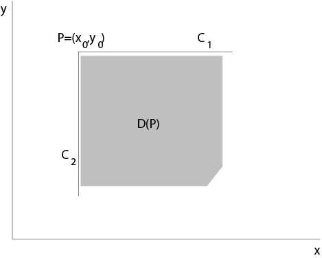
Figure 4.4.2: Definition of Riemann's function

$$\begin{eqnarray} \label{riem9} Mv&=&0\ \ \mbox{in}\ D(P)\\ \label{riem10} bv-v_x&=&0\ \ \mbox{on}\ C_1\\ \label{riem11} av-v_y&=&0\ \ \mbox{on}\ C_2\\ \label{riem12} v(P)&=&1. \end{eqnarray}$$

Assume $v$ satisfies ($\ref{riem9}$)-($\ref{riem12}$), then

$$\begin{eqnarray*} 2u(P)&=&u(A)v(A)+u(B)v(B)-2\int_\Omega\ fv\ dxdy\\ &&=\int_{BA}(u_xv-v_x+2buv)\ dx-(u_yv-v_yu+2auv)\ dy, \end{eqnarray*}$$

where the right hand side is known from given data.

A function $v=v(x,y;x_0,y_0)$ satisfying ($\ref{riem9}$)-($\ref{riem12}$) is called Riemann's function.

Remark. Set $w(x,y)=v(x,y;x_0,y_0)$ for fixed $x_0,\ y_0$. Then ($\ref{riem9}$)-($\ref{riem12}$) imply

$$\begin{eqnarray*} w(x,y_0)&=&\exp\left(\int_{x_0}^x\ b(\tau,y_0)\ d\tau\right)\ \ \mbox{on}\ C_1,\\ w(x_0,y)&=&\exp\left(\int_{y_0}^y\ a(x_0,\tau)\ d\tau\right)\ \ \mbox{on}\ C_2. \end{eqnarray*}$$

Example 4.4.1:

$u_{xy}=f(x,y)$, then a Riemann function is $v(x,y)\equiv 1$.

Example 4.4.2:

Consider the telegraph equation of Chapter 3

$$\varepsilon \mu u_{tt}=c^2\triangle_xu-\lambda\mu u_t,\]

where $u$ stands for one coordinate of electric or magnetic field.

Introducing

$$u=w(x,t)e^{\kappa t},\]

where $\kappa=-\lambda/(2\varepsilon)$, we arrive at

$$w_{tt}=\frac{c^2}{\varepsilon\mu}\triangle_xw-\frac{\lambda^2}{4\epsilon^2}.\]

Stretching the axis and transform the equation to the normal form we get finally the following equation, the new function is denoted by $u$ and the new variables are denoted by $x,y$ again,

$$u_{xy}+cu=0,\]

with a positive constant $c$. We make the ansatz for a Riemann function

$$v(x,y;x_0,y_0)=w(s),\ \ s=(x-x_0)(y-y_0)\]

and obtain

$$sw''+w'+cw=0.\]

Substitution $\sigma=\sqrt{4cs}$ leads to Bessel's differential equation

$$\sigma^2 z''(\sigma)+\sigma z'(\sigma)+\sigma^2 z(\sigma)=0,\]

where $z(\sigma)=w(\sigma^2/(4c))$. A solution is

$$J_0(\sigma)=J_0\left(\sqrt{4c(x-x_0)(y-y_0)}\right)\]

which defines a Riemann function since $J_0(0)=1$.

Remark. Bessel's differential equation is

$$x^2y''(x)+xy'(x)+(x^2-n^2)y(x)=0,\]

where $n\in\mathbb{R}^1$. If $n\in{\mathbb N}\cup\{0\}$, then solutions are given by Bessel functions. One of the two linearly independent solutions is bounded at 0. This bounded solution is the Bessel function $J_n(x)$ of first kind and of order $n$, see [1], for example.

Contributors and Attributions

• Prof. Dr. Erich Miersemann (Universität Leipzig)

• Integrated by Justin Marshall.