4.8: Inverse Functions

Last updated
Save as PDF

Page ID: 40921

$ \newcommand{\vecs}[1]{\overset { \scriptstyle \rightharpoonup} {\mathbf{#1}} } $ $ \newcommand{\vecd}[1]{\overset{-\!-\!\rightharpoonup}{\vphantom{a}\smash {#1}}} $$\newcommand{\id}{\mathrm{id}}$ $ \newcommand{\Span}{\mathrm{span}}$ $ \newcommand{\kernel}{\mathrm{null}\,}$ $ \newcommand{\range}{\mathrm{range}\,}$ $ \newcommand{\RealPart}{\mathrm{Re}}$ $ \newcommand{\ImaginaryPart}{\mathrm{Im}}$ $ \newcommand{\Argument}{\mathrm{Arg}}$ $ \newcommand{\norm}[1]{\| #1 \|}$ $ \newcommand{\inner}[2]{\langle #1, #2 \rangle}$ $ \newcommand{\Span}{\mathrm{span}}$ $\newcommand{\id}{\mathrm{id}}$ $ \newcommand{\Span}{\mathrm{span}}$ $ \newcommand{\kernel}{\mathrm{null}\,}$ $ \newcommand{\range}{\mathrm{range}\,}$ $ \newcommand{\RealPart}{\mathrm{Re}}$ $ \newcommand{\ImaginaryPart}{\mathrm{Im}}$ $ \newcommand{\Argument}{\mathrm{Arg}}$ $ \newcommand{\norm}[1]{\| #1 \|}$ $ \newcommand{\inner}[2]{\langle #1, #2 \rangle}$ $ \newcommand{\Span}{\mathrm{span}}$$\newcommand{\AA}{\unicode[.8,0]{x212B}}$

An inverse function undoes the action of the original function. So the inverse of a function that squared a number would be a function that square rooted a number. In general, an inverse function will take a $y$ value from the original function and return the $x$ value that produced it.

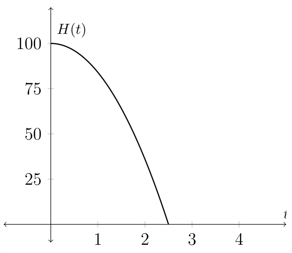
We can see this in an application. Given an object with little or no air resistance that is dropped from $100 \mathrm{ft}$, the function that describes its height as a function of time would be:
\[
H(t)=100-16 t^{2}
\]
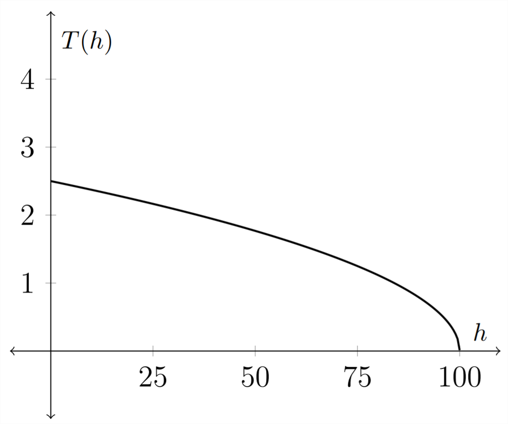
In this function, $H(t)$ is the height of the object at time $t .$ If we wanted to turn this around so that it described the time for a given height, then we would want to isolate the $t$ variable. In this example, the graph of the function would change in that the original independent variable - $t,$ becomes the dependent variable in the inverse function.
\[
\begin{aligned}
h &=100-16 t^{2} \\
16 t^{2} &=100-h \\
t^{2} &=\frac{100-h}{16} \\
t &=\sqrt{\frac{100-h}{16}} \\
T(h) &=\frac{\sqrt{100-h}}{4}
\end{aligned}
\]

Original function: $H(t)=100-16 t^{2}$
$clipboard_e3860268f9d6975d40696f81c10a4e402.png$
Inverse function: $T(h)=\frac{\sqrt{100-h}}{4}$
$clipboard_e89256480f8675d2b57ce0801450f241e.png$
Notice that the graph of the function inverse is the original function reflected over the line $y=x,$ because an inverse function interchanges the independent and dependent variables.

Finding a formula for an inverse function can be more confusing when we consider a standard function $y=f(x) .$ In our standard notation, $x$ is always considered to be the independent variable and $y$ is always considered to be the dependent variable.

Notice in the example above that when we graphed the function and its inverse, the label on the $x$ axis changed from $t$ to $h .$ In a standard function, the $x$ axis will always be the $x$ axis and the $y$ axis will always be the $y$ axis. To compensate for this, when we find a function inverse for a function stated in terms of $x$ and $y$ we generally interchange the $x$ and $y$ terms so that $x$ remains the independent variable.
In our example, we had
\[
H(t)=100-16 t^{2}
\]
and found the inverse to be
\[
T(h)=\frac{\sqrt{100-h}}{4}
\]
If the original function had been stated in terms of $x$ and $y,$ then the process would have looked like this:
\begin{aligned}
f(x) &=100-16 x^{2} \\
y &=100-16 x^{2} \\
16 x^{2} &=100-y \\
x^{2} &=\frac{100-y}{16} \\
x &=\sqrt{\frac{100-y}{16}} \\
x &=\frac{\sqrt{100-y}}{4}
\end{aligned}

Then we switch the $x$ and $y$ variables to keep the $x$ as the independent variable:
\[
y=f^{-1}(x)=\frac{\sqrt{100-x}}{4}
\]
$\mathrm{So}$
\[
f(x)=100-16 x^{2}
\]
and
\[
f^{-1}(x)=\frac{\sqrt{100-x}}{4}
\]

Exercises 4.8
Given the function $f(x),$ find the inverse function $f^{-1}(x)$
1) $\quad f(x)=3 x$
2) $\quad f(x)=-4 x$
3) $\quad f(x)=4 x+2$
4) $\quad f(x)=1-3 x$
5) $\quad f(x)=x^{3}-1$
6) $\quad f(x)=x^{3}+1$
7) $\quad f(x)=x^{2}+4 (x \geq 4)$
8) $\quad f(x)=x^{2}+9 (x \geq 9)$
9) $\quad f(x)=\frac{4}{x}$
10) $\quad f(x)=-\frac{3}{x}$
11) $\quad f(x)=\frac{1}{x-2}$
12) $\quad f(x)=\frac{4}{x+2}$
13) $\quad f(x)=\frac{2}{x+3}$
14) $\quad f(x)=\frac{4}{2-x}$
15) $\quad f(x)=\frac{3 x}{x+2}$
16) $\quad f(x)=-\frac{2 x}{x-1}$
17) $\quad f(x)=\frac{2 x}{3 x-1}$
18) $\quad f(x)=-\frac{3 x+1}{x}$
19) $\quad f(x)=\frac{3 x+4}{2 x-3}$
20) $\quad f(x)=\frac{2 x-3}{x+4}$
21) $\quad f(x)=\frac{2 x+3}{x+2}$
22) $\quad f(x)=-\frac{3 x+4}{x-2}$
Find the inverse function for each of the following applications.
23) The volume of water left in a 1000 gallon tank that drains in 40 minutes is modeled by the equation:
\[
V(t)=1000\left(1-\frac{t}{40}\right)^{2}
\]
Find $T(v)$ - the function that tells you how long the water has been draining given a particular volume left in the tank. Time is measured in minutes and the volume is measured in gallons.
24) The speed of a vehicle in miles per hour that leaves skid marks $d$ feet long is modeled by the equation:
\[
R(d)=2 \sqrt{5 d}
\]
Find $D(r)$ - the function that tells you the stopping distance for a vehicle traveling $r$ miles per hour.
25) The period of a pendulum of length $\ell$ can be expressed by the relationship:
\[
T(\ell)=2 \pi \sqrt{\frac{\ell}{980}}
\]
Find the function $L(t)$ that determines the length of a pendulum given its period. Here the time is measured in seconds and the length is measured in centimeters.
26) The volume of a sphere of radius $r$ is given by the formula:
\[
V(r)=\frac{4}{3} \pi r^{3}
\]
Find $R(v)$ - the function that determines the radius of a sphere given its volume.