2.4: Solving Equations and Inequalities by Graphing

Our emphasis in the chapter has been on functions and the interpretation of their graphs. In this section, we continue in that vein and turn our exploration to the solution of equations and inequalities by graphing. The equations will have the form \(f(x) = g(x)\), and the inequalities will have form \(f(x) < g(x)\) and/or \(f(x) > g(x)\).

You might wonder why we have failed to mention inequalities having the form \(f(x) \leq g(x)\) and \(f(x) \geq g(x)\). The reason for this omission is the fact that the solution of the inequality \(f(x) \leq g(x)\) is simply the union of the solutions of \(f(x) = g(x)\) and \(f(x) < g(x)\). After all, \(\leq\) is pronounced “less than or equal.” Similar comments are in order for the inequality \(f(x) \geq g(x)\).

We will begin by comparing the function values of two functions f and g at various values of x in their domains.

Comparing Functions

Suppose that we evaluate two functions f and g at a particular value of x. One of three outcomes is possible. Either

\[f(x)=g(x), \quad \text { or } \quad f(x)>g(x), \quad \text { or } \quad f(x)<g(x) \nonumber \]

It’s pretty straightforward to compare two function values at a particular value if rules are given for each function.

Example \(\PageIndex{1}\)

Given \(f(x)=x^{2}\) and \(g(x) = 2x+3\), compare the functions at x = −2, 0, and 3.

Solution

Simple calculations reveal the relations.

• At x = −2, \[f(-2)=(-2)^{2}=4 \quad \text { and } \quad g(-2)=2(-2)+3=-1 \nonumber \] so clearly, \(f(−2) > g(−2)\).
• At x = 0, \[f(0)=(0)^{2}=0 \quad \text { and } \quad g(0)=2(0)+3=3 \nonumber \] so clearly, \(f(0) < g(0)\).
• Finally, at x = 3, \[f(3)=(3)^{2}=9 \quad \text { and } \quad g(3)=2(3)+3=9 \nonumber \] so clearly, \(f(3) = g(3)\).

We can also compare function values at a particular value of x by examining the graphs of the functions. For example, consider the graphs of two functions f and g in Figure \(\PageIndex{1}\).

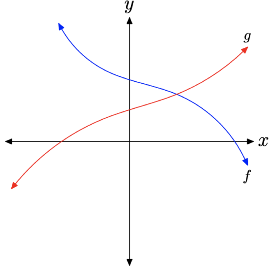
Figure \(\PageIndex{1}\)

Next, suppose that we draw a dashed vertical line through the point of intersection of the graphs of f and g, then select a value of x that lies to the left of the dashed vertical line, as shown in Figure \(\PageIndex{2}\)(a). Because the graph of f lies above the graph of g for all values of x that lie to the left of the dashed vertical line, it will be the case that \(f(x) > g(x)\) for all such x (see Figure \(\PageIndex{2}\)(a)).

On the other hand, the graph of f lies below the graph of g for all values of x that lie to the right of the dashed vertical line. Hence, for all such x, it will be the case that \(f(x) < g(x)\) (see Figure \(\PageIndex{2}\)(b)).

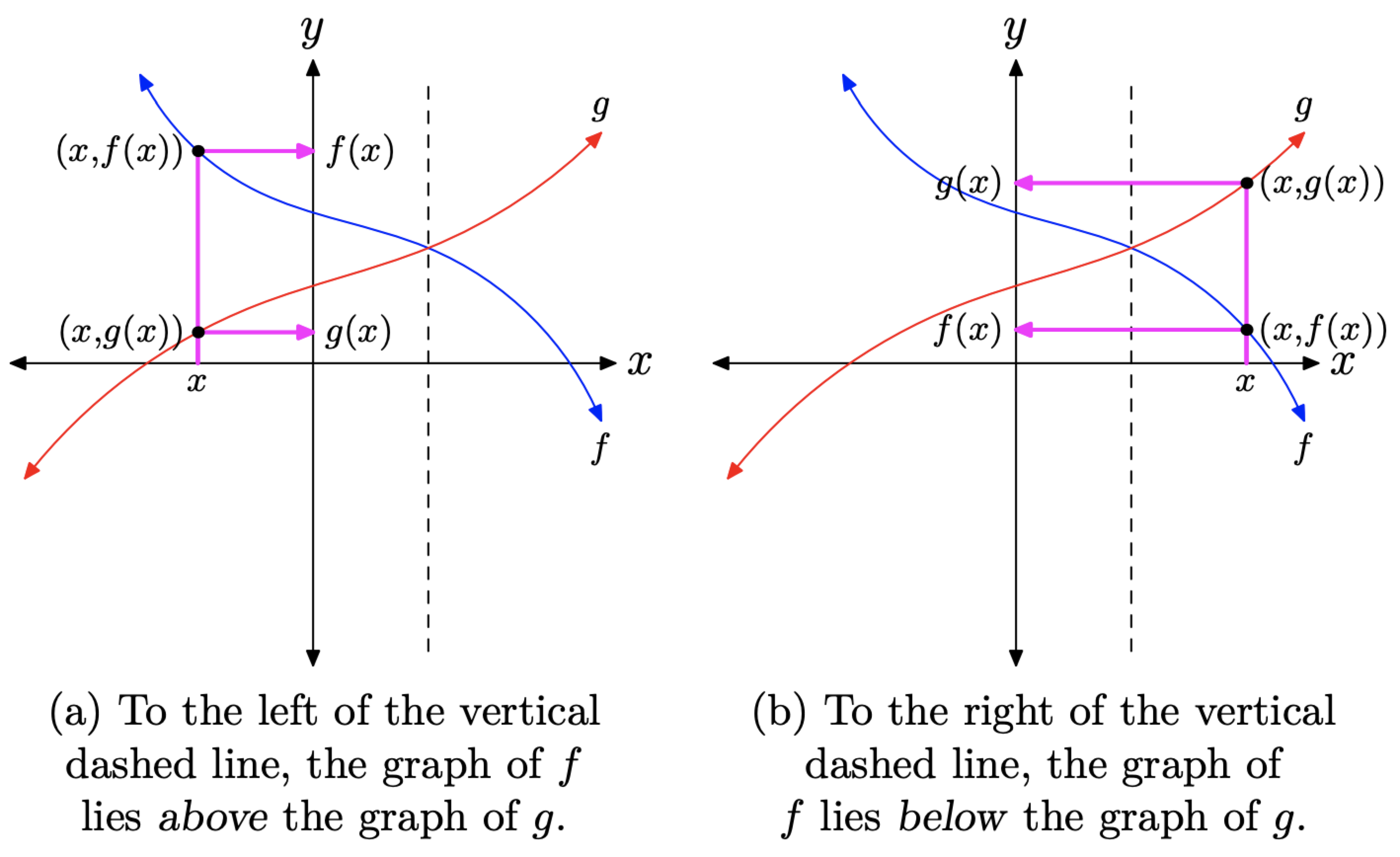
Figure \(\PageIndex{2}\). Comparing f and g.

Finally, if we select the x-value of the point of intersection of the graphs of f and g, then for this value of x, it is the case that f(x) and g(x) are equal; that is, \(f(x) = g(x)\) (see Figure \(\PageIndex{3}\)).

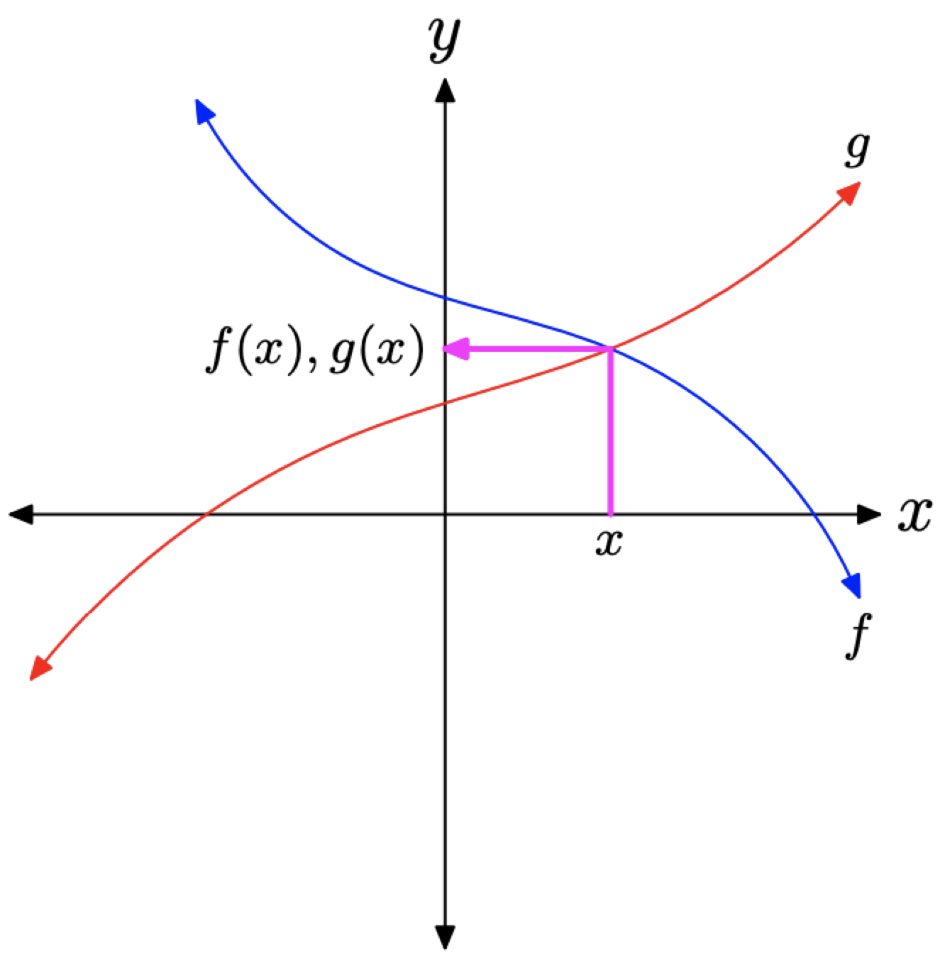
Figure \(\PageIndex{3}\). The function values f(x) and g(x) are equal where the graphs of f and g intersect.

Let’s summarize our findings.

Summary

1. The solution of the equation f(x) = g(x) is the set of all x for which the graphs of f and g intersect.
2. The solution of the inequality f(x) < g(x) is the set of all x for which the graph of f lies below the graph of g.
3. The solution of the inequality f(x) > g(x) is the set of all x for which the graph of f lies above the graph of g.

Let’s look at an example.

Example \(\PageIndex{2}\)

Given the graphs of f and g in Figure \(\PageIndex{4}\)(a), use both set-builder and interval notation to describe the solution of the inequality f(x) < g(x). Then find the solutions of the inequality f(x) > g(x) and the equation f(x) = g(x) in a similar fashion.

Solution

To find the solution of f(x) < g(x), we must locate where the graph of f lies below the graph of g. We draw a dashed vertical line through the point of intersection of the graphs of f and g (see Figure \(\PageIndex{4}\)(b)), then note that the graph of f lies below the graph of g to the left of this dashed line. Consequently, the solution of the inequality f(x) < g(x) is the collection of all x that lie to the left of the dashed line. This set is shaded in red (or in a thicker line style if viewing in black and white) on the x-axis in Figure \(\PageIndex{4}\)(b).

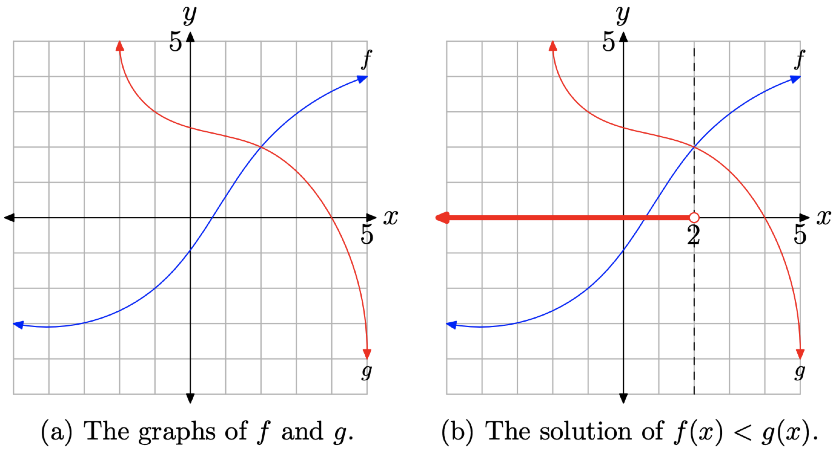
Figure \(\PageIndex{4}\). Comparing f and g.

Note that the shaded points on the x-axis have x-values less than 2. Hence, the solution of f(x) < g(x) is \[(-\infty, 2)=\{x : x<2\} \nonumber \]

In like manner, the solution of f(x) > g(x) is found by noting where the graph of f lies above the graph of g and shading the corresponding x-values on the x-axis (see Figure \(\PageIndex{5}\)(a)). The solution of f(x) > g(x) is \((2, \infty)\), or alternatively, \(\{x : x>2\}\).

To find the solution of f(x) = g(x), note where the graph of f intersects the graph of g, then shade the x-value of this point of intersection on the x-axis (see Figure \(\PageIndex{5}\)(b)). Therefore, the solution of f(x) = g(x) is \(\{x : x = 2\}\). This is not an interval, so it is not appropriate to describe this solution with interval notation.

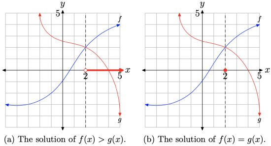
Figure \(\PageIndex{5}\). Further comparisons.

Let’s look at another example.

Example \(\PageIndex{3}\)

Given the graphs of f and g in Figure \(\PageIndex{6}\)(a), use both set-builder and interval notation to describe the solution of the inequality f(x) > g(x). Then find the solutions of the inequality f(x) < g(x) and the equation f(x) = g(x) in a similar fashion.

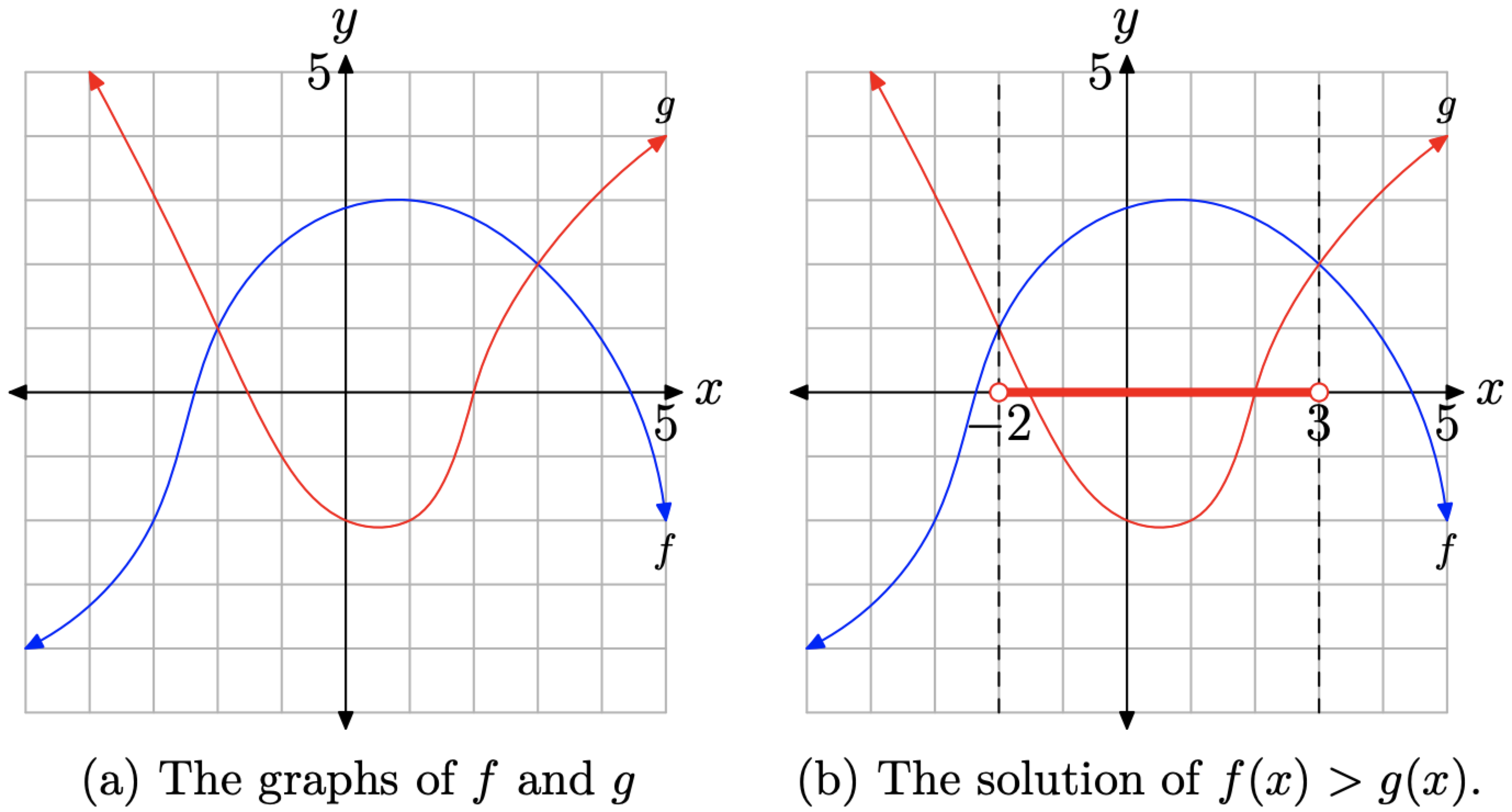
Figure \(\PageIndex{6}\). Comparing f and g.

Solution

To determine the solution of f(x) > g(x), we must locate where the graph of f lies above the graph of g. Draw dashed vertical lines through the points of intersection of the graphs of f and g (see Figure \(\PageIndex{6}\)(b)), then note that the graph of f lies above the graph of g between the dashed vertical lines just drawn. Consequently, the solution of the inequality f(x) > g(x) is the collection of all x that lie between the dashed vertical lines. We have shaded this collection on the x-axis in red (or with a thicker line style for those viewing in black and white) in Figure \(\PageIndex{6}\)(b).

Note that the points shaded on the x-axis in Figure \(\PageIndex{6}\)(b) have x-values between −2 and 3. Consequently, the solution of f(x) > g(x) is

\[(-2,3)=\{x :-2<x<3\} \nonumber \]

In like manner, the solution of f(x) < g(x) is found by noting where the graph of f lies below the graph of g and shading the corresponding x-values on the x-axis (see Figure 7(a)). Thus, the solution of f(x) < g(x) is

\[(-\infty,-2) \cup(3, \infty)=\{x : x<-2 \text { or } x>3\} \nonumber \]

To find the solution of f(x) = g(x), note where the graph of f intersects the graph of g, and shade the x-value of each point of intersection on the x-axis (see Figure \(\PageIndex{7}\)(b)). Therefore, the solution of f(x) = g(x) is \(\{x : x=-2\) or \(x=3\}\). Because this solution set is not an interval, it would be inappropriate to describe it with interval notation.

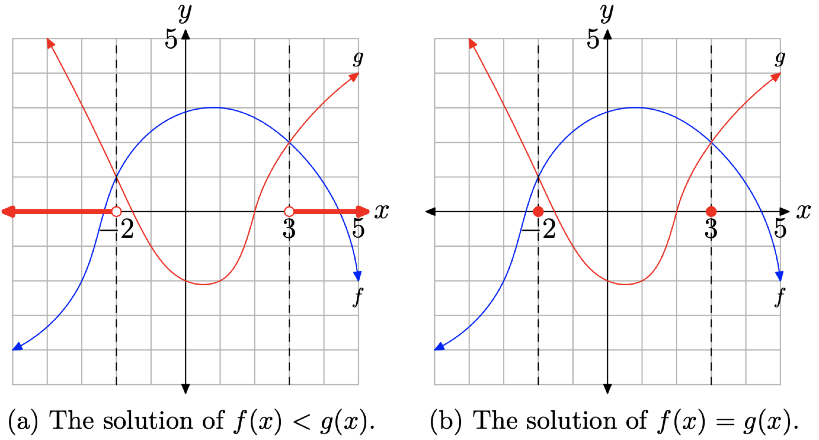
Figure \(\PageIndex{7}\). Further comparisons.

Solving Equations and Inequalities with the Graphing Calculator

We now know that the solution of f(x) = g(x) is the set of all x for which the graphs of f and g intersect. Therefore, the graphing calculator becomes an indispensable tool when solving equations.

Example \(\PageIndex{4}\)

Use a graphing calculator to solve the equation

\[1.23 x-4.56=5.28-2.35 x \qquad (6) \nonumber \]

Solution

Note that equation (6) has the form f(x) = g(x), where

\[f(x)=1.23 x-4.56 \quad \text { and } \quad g(x)=5.28-2.35 x \nonumber \]

Thus, our approach will be to draw the graphs of f and g, then find the x-value of the point of intersection.

First, load f(x) = 1.23x − 4.56 into Y1 and g(x) = 5.28 − 2.35x into Y2 in the Y= menu of your graphing calculator (see Figure \(\PageIndex{8}\)(a)). Select 6:ZStandard in the ZOOM menu to produce the graphs in Figure \(\PageIndex{8}\)(b).

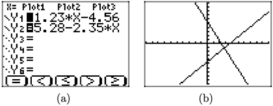
Figure \(\PageIndex{8}\). Sketching the graphs of f(x) = 1.23x−4.56 and g(x) = 5.28 − 2.35x.

The solution of equation (6) is the x-value of the point of intersection of the graphs of f and g in Figure (\PageIndex{8}\)(b). We will use the intersect utility in the CALC menu on the graphing calculator to determine the coordinates of the point of intersection.

We proceed as follows:

• Select 2nd CALC (push the 2nd button, followed by the TRACE button), which opens the menu shown in Figure (\PageIndex{9}\)(a).
• Select 5:intersect. The calculator responds by placing the cursor on one of the graphs, then asks if you want to use the selected curve. You respond in the affirmative by pressing the ENTER key on the calculator.
• The calculator responds by placing the cursor on the second graph, then asks if you want to use the selected curve. Respond in the affirmative by pressing the ENTER key.
• The calculator responds by asking you to make a guess. In this case, there are only two graphs on the calculator, so any guess is appropriate.4 Simply press the ENTER key to use the current position of the cursor as your guess.

Figure \(\PageIndex{9}\). Using the intersect utility.

The result of this sequence of steps is shown in Figure \(\PageIndex{10}\). The coordinates of the point of intersection are approximately (2.7486034, −1.179218). The x-value of this point of intersection is the solution of equation (6). That is, the solution of \(1.23x − 4.56 = 5.28 − 2.35x\) is approximately \(x \approx 2.7486034\).

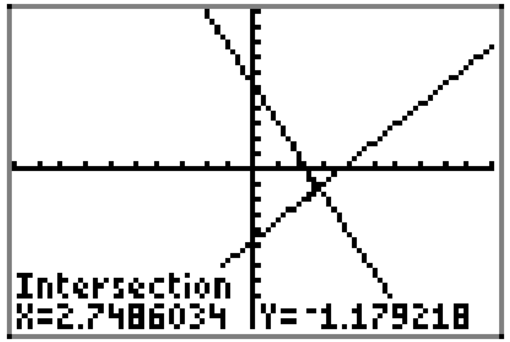
Figure \(\PageIndex{10}\). The coordinates of the point of intersection.

Summary

Guidelines.

You’ll need to discuss expectations with your teacher, but we expect our students to summarize their results as follows.

1. Set up a coordinate system.6 Label and scale each axis with xmin, xmax, ymin, and ymax.

2. Copy the image in your viewing window onto your coordinate system. Label each graph with its equation.

3. Draw a dashed vertical line through the point of intersection.

4. Shade and label the solution of the equation on the x-axis.

The result of following this standard is shown in Figure \(\PageIndex{11}\).

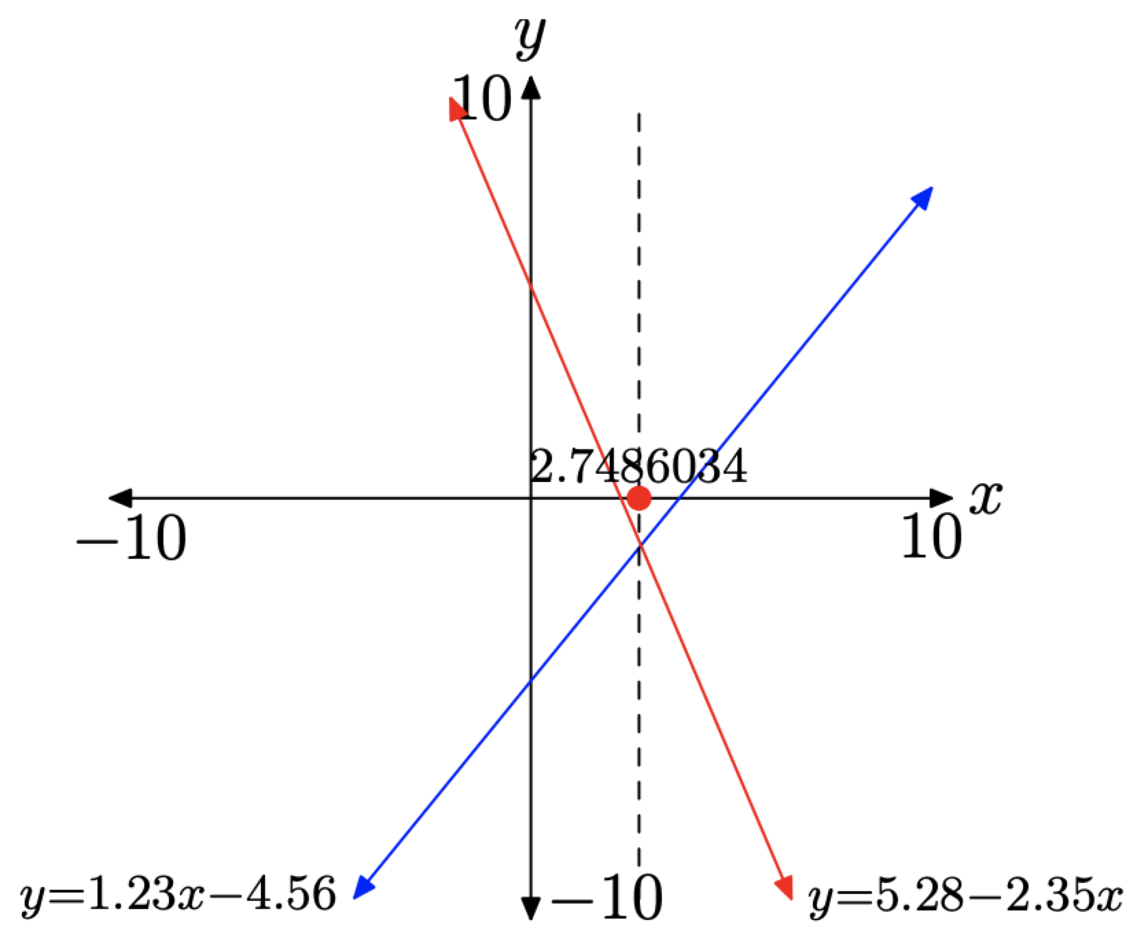
Figure \(\PageIndex{11}\). Summarizing the solution of equation (6).

Let’s look at another example.

Example \(\PageIndex{5}\)

Use set-builder and interval notation to describe the solution of the inequality

\[0.85 x^{2}-3 \geq 1.23 x+1.25 \qquad (9) \nonumber \]

Solution

Note that the inequality (9) has the form \(f(x) \geq g(x)\), where

\[f(x)=0.85 x^{2}-3 \quad \text { and } \quad g(x)=1.23 x+1.25 \nonumber \]

Load \(f(x)=0.85 x^{2}-3\) and \(g(x)=1.23 x+1.25\) into Y1 and Y2 in the Y= menu, respectively, as shown in Figure \(\PageIndex{12}\)(a). Select 6:ZStandard from the ZOOM menu to produce the graphs shown in Figure \(\PageIndex{12}\)(b).

To find the points of intersection of the graphs of f and g, we follow the same sequence of steps as we did in Example \(\PageIndex{4}\) up to the point where the calculator asks you to make a guess (i.e., 2nd CALC, 5:intersect, First curve ENTER, Second curve ENTER). Because there are two points of intersection, when the calculator asks you to

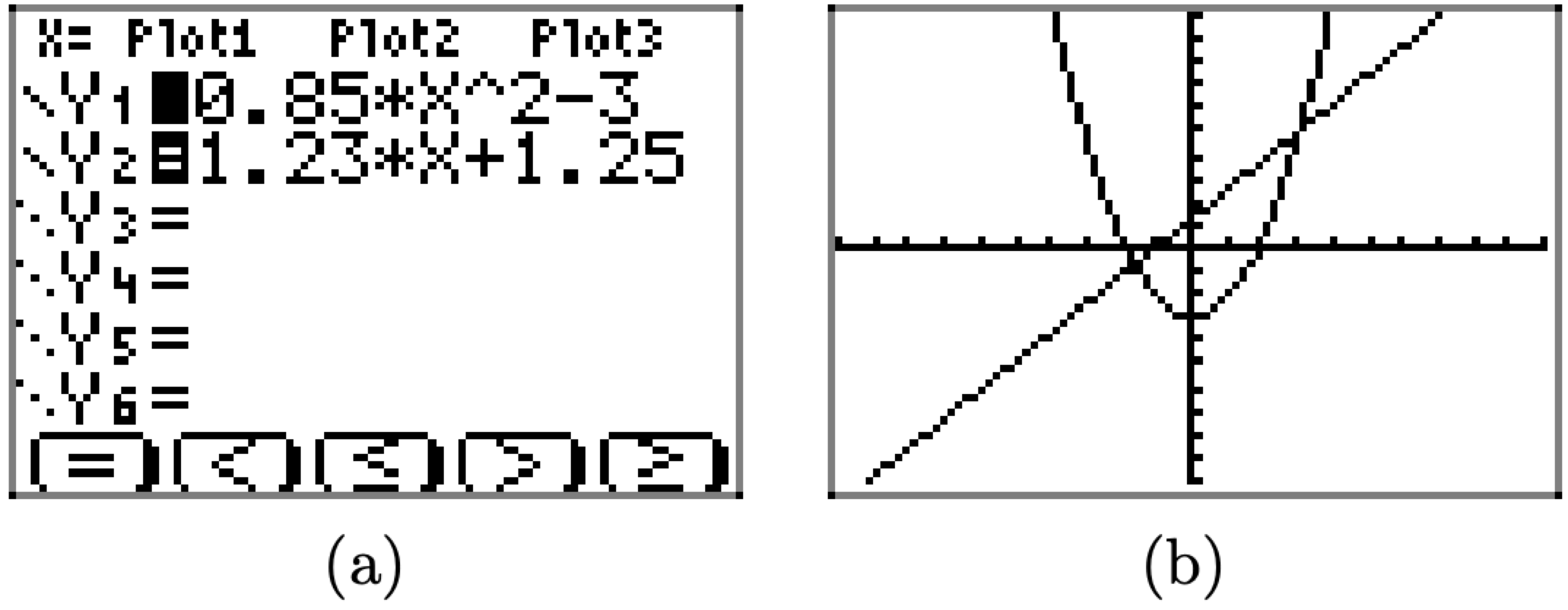
Figure \(\PageIndex{12}\). The graphs of \(f(x)=0.85 x^{2}-3\) and \(g(x) = 1.23x + 1.25\).

make a guess, you must move your cursor (with the arrow keys) so that it is closer to the point of intersection you wish to find than it is to the other point of intersection. Using this technique produces the two points of intersection found in Figures \(\PageIndex{13}\)(a) and (b).

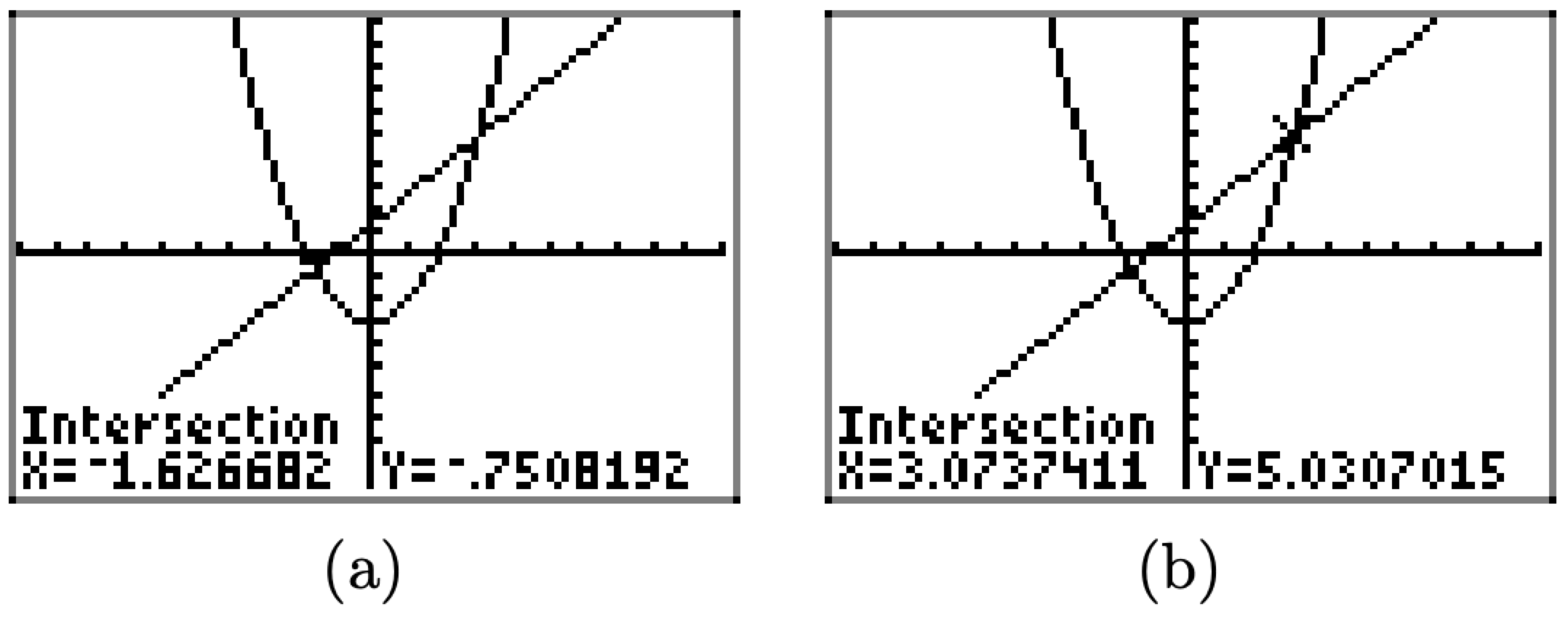
Figure \(\PageIndex{13}\). The points of intersection of the graphs of f and g.

The approximate coordinates of the first point of intersection are (−1.626682, −0.7508192). The second point of intersection has approximate coordinates (3.0737411, 5.0307015).

It is important to remember that every time you pick up your calculator, you are only getting an approximation. It is possible that you will get a slightly different result for the points of intersection. For example, you might get (−1.626685, −0.7508187) for your point of intersection. Based on the position of the cursor when you marked the curves and made your guess, you can get slightly different approximations. Note that this second solution is very nearly the same as the one we found, differing only in the last few decimal places, and is perfectly acceptable as an answer.

We now summarize our results by creating a coordinate system, labeling the axes, and scaling the axes with the values of the window parameters xmin, xmax, ymin, and ymax. We copy the image in our viewing window onto this coordinate system, labeling each graph with its equation. We then draw dashed vertical lines through each point of intersection, as shown in Figure \(\PageIndex{14}\).

We are solving the inequality \(0.85 x^{2}-3 \geq 1.23 x+1.25\). The solution will be the union of the solutions of \(0.85 x^{2}-3>1.23 x+1.25\) and \(0.85 x^{2}-3=1.23 x+1.25\).

• To solve \(0.85 x^{2}-3>1.23 x+1.25\), we note where the graph of \(y=0.85 x^{2}-3\) lies above the graph of \(y=1.23 x+1.25\) and shade the corresponding x-values

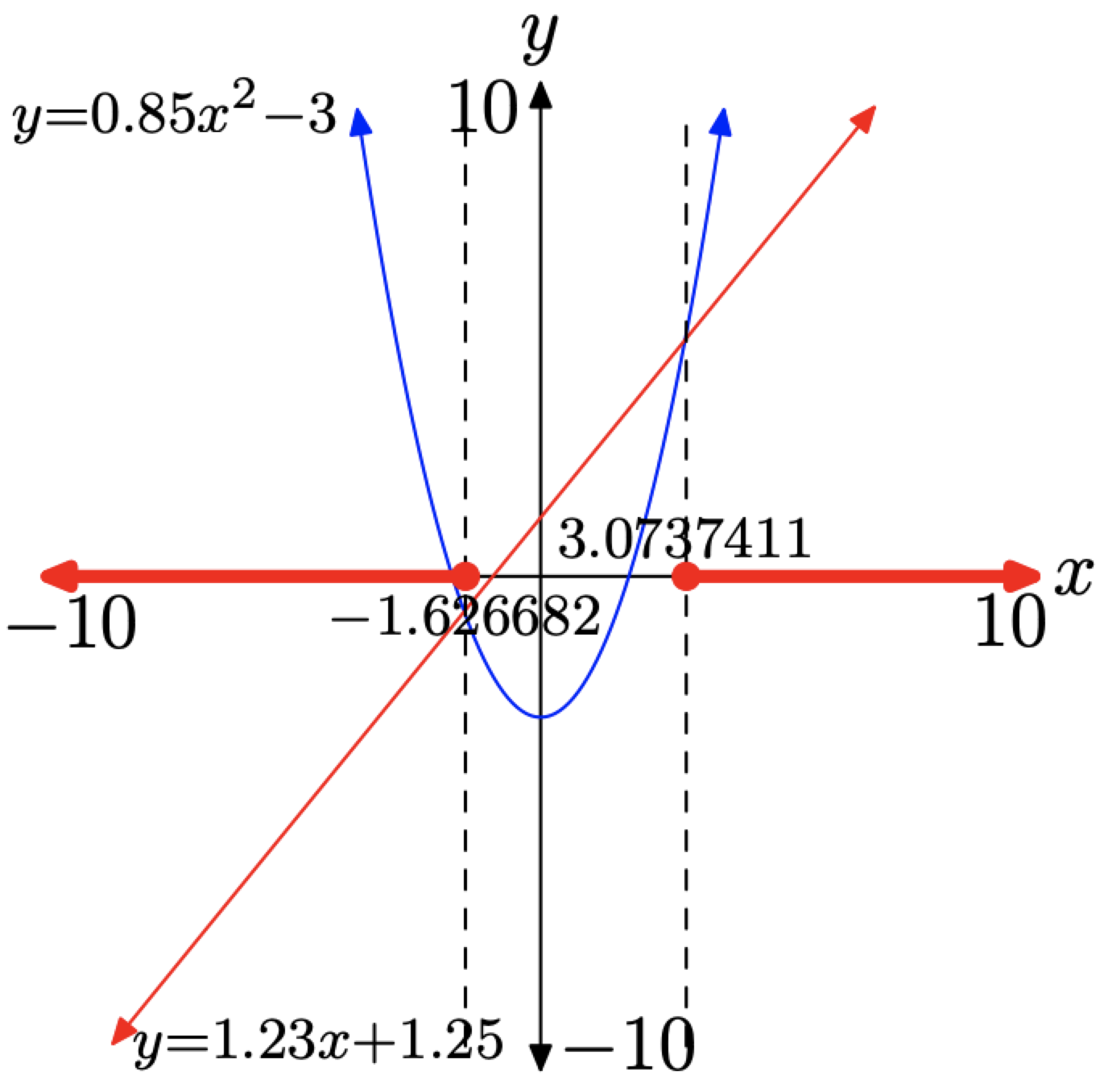
Figure \(\PageIndex{14}\). Summarizing the solution of \(0.85 x^{2}-3 \geq 1.23 x+1.25\).

on the x-axis. In this case, the graph of \(y=0.85 x^{2}-3\) lies above the graph of \(y=1.23 x+1.25\) for values of x that lie outside of our dashed vertical lines.

• To solve \(0.85 x^{2}-3=1.23 x+1.25\), we note where the graph of \(y=0.85 x^{2}-3\) intersects the graph of \(y = 1.23x + 1.25\) and shade the corresponding x-values on the x-axis. This is why the points at \(x \approx-1.626682\) and \(x \approx 3.0737411\) are “filled.”

Thus, all values of x that are either less than or equal to −1.626682 or greater than or equal to 3.0737411 are solutions. That is, the solution of inequality \(0.85x^{2} − 3 > 1.23x + 1.25\) is approximately

\[(-\infty,-1.626682] \cup[3.0737411, \infty)=\{x : x \leq-1.626682 \text { or } x \geq 3.0737411\} \nonumber \]

Comparing Functions with Zero

When we evaluate a function f at a particular value of x, only one of three outcomes is possible. Either

\[f(x)=0, \quad \text { or } \quad f(x)>0, \quad \text { or } \quad f(x)<0 \nonumber \]

That is, either f(x) equals zero, or f(x) is positive, or f(x) is negative. There are no other possibilities.

We could start fresh, taking a completely new approach, or we can build on what we already know. We choose the latter approach. Suppose that we are asked to compare f(x) with zero? Is it equal to zero, is it greater than zero, or is it smaller than zero?

We set g(x) = 0. Now, if we want to compare the function f with zero, we need only compare f with g, which we already know how to do. To find where f(x) = g(x), we note where the graphs of f and g intersect, to find where f(x) > g(x), we note where the graph of f lies above the graph of g, and finally, to find where f(x) < g(x), we simply note where the graph of f lies below the graph of g.

However, the graph of g(x) = 0 is a horizontal line coincident with the x-axis. Indeed, g(x) = 0 is the equation of the x-axis. This argument leads to the following key results.

summary

• The solution of f(x) = 0 is the set of all x for which the graph of f intersects the x-axis.
• The solution of f(x) > 0 is the set of all x for which the graph of f lies strictly above the x-axis.
• The solution of f(x) < 0 is the set of all x for which the graph of f lies strictly below the x-axis.

For example:

• To find the solution of f(x) = 0 in Figure \(\PageIndex{15}\)(a), we simply note where the graph of f crosses the x-axis in Figure \(\PageIndex{15}\)(a). Thus, the solution of f(x) = 0 is x = 1.
• To find the solution of f(x) > 0 in Figure \(\PageIndex{15}\)(b), we simply note where the graph of f lies above the x-axis in Figure \(\PageIndex{15}\)(b), which is to the right of the vertical dashed line through x = 1. Thus, the solution of f(x) > 0 is \((1, \infty)=\{x : x>1\}\).
• To find the solution of f(x) < 0 in Figure \(\PageIndex{15}\)(c), we simply note where the graph of f lies below the x-axis in Figure \(\PageIndex{15}\)(c), which is to the left of the vertical dashed line at x = 1. Thus, the solution of f(x) < 0 is \((-\infty, 1)=\{x : x<1\}\).

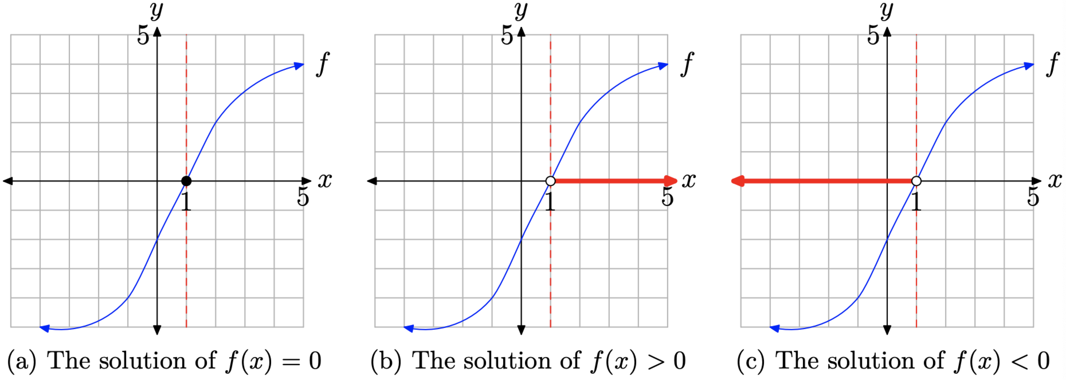
Figure \(\PageIndex{15}\). Comparing the function f with zero.

We next define some important terminology.

Definition

If f(a) = 0, then a is called a zero of the function f. The graph of f will intercept the x-axis at \((a, 0)\), a point called the x-intercept of the graph of f.

Your calculator has a utility that will help you to find the zeros of a function.

Example \(\PageIndex{6}\)

Use a graphing calculator to solve the inequality

\[0.25 x^{2}-1.24 x-3.84 \leq 0 \nonumber \]

Solution

Note that this inequality has the form \(f(x) \leq 0\), where \(f(x)=0.25 x^{2}-1.24 x-3.84\). Our strategy will be to draw the graph of f, then determine where the graph of f lies below or on the x-axis.

We proceed as follows:

• First, load the function f(x) = 0.25x 2 − 1.24x − 3.84 into the Y1 in the Y= menu of your calculator. Select 6:ZStandard from the ZOOM menu to produce the image in Figure \(\PageIndex{16}\)(a).
• Press 2nd CALC to open the menu shown in Figure \(\PageIndex{16}\)(b), then select 2:zero to start the utility that will find a zero of the function (an x-intercept of the graph).
• The calculator asks for a “Left Bound,” so use your arrow keys to move the cursor slightly to the left of the leftmost x-intercept of the graph, as shown in Figure \(\PageIndex{16}\)(c). Press ENTER to record this “Left Bound.”
• The calculator then asks for a “Right Bound,” so use your arrow keys to move the cursor slightly to the right of the x-intercept, as shown in Figure \(\PageIndex{16}\)(d). Press ENTER to record this “Right Bound.”

Figure (\PageIndex{16}\). Finding a zero or x-intercept with the calculator.

• The calculator responds by marking the left and right bounds on the screen, as shown in Figure (\PageIndex{17}\)(a), then asks you to make a reasonable starting guess for the zero or x-intercept. You may use the arrow keys to move your cursor to any point, so long as the cursor remains between the left- and right-bound marks on the viewing window. We usually just leave the cursor where it is and press the ENTER to record this guess. We suggest you do that as well.
• The calculator responds by finding the coordinates of the x-intercept, as shown in Figure (\PageIndex{17}\)(b). Note that the x-coordinate of the x-intercept is approximately −2.157931.
• Repeat the procedure to find the coordinates of the rightmost x-intercept. The result is shown in Figure (\PageIndex{17}\)(c). Note that the x-coordinate of the intercept is approximately 7.1179306.

The final step is the interpretation of results and recording of our solution on our homework paper. Referring to the Summary 7 Guidelines, we come up with the graph shown in Figure (\PageIndex{18}\).

Figure (\PageIndex{17}\). Finding a zero or x-intercept with the calculator.

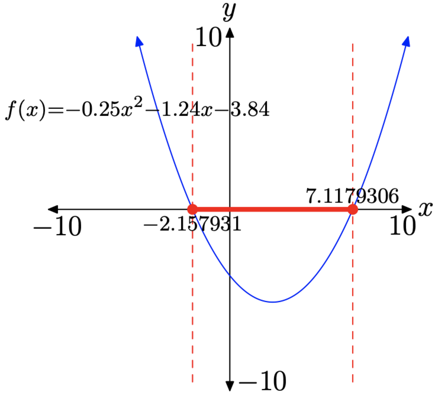
Figure (\PageIndex{18}\). The solution of \(0.25 x^{2}- 1.24 x-3,84 \leq 0 .\).

Several comments are in order. Noting that \(f(x)=0.25 x^{2}-1.24 x-3.84\), we note:

1. The solutions of f(x) = 0 are the points where the graph crosses the x-axis. That’s why the points (−2.157931, 0) and (7.1179306, 0) are shaded and filled in Figure (\PageIndex{18}\).
2. The solutions of f(x) < 0 are those values of x for which the graph of f falls strictly below the x-axis. This occurs for all values of x between −2.157931 and 7.1179306. These points are also shaded on the x-axis in Figure (\PageIndex{18}\).
3. Finally, the solution of \(f(x) \leq 0\) is the union of these two shadings, which we describe in interval and set-builder notation as follows:

\[[-2.157931,7.1179306]=\{x :-2.157931 \leq x \leq 7.1179306\} \nonumber \]