2.6: Horizontal Transformations

In the previous section, we introduced the concept of transformations. We made a change to the basic equation y = f(x), such as y = af(x), y = −f(x), y = f(x) − c, or y = f(x) + c, then studied how these changes affected the shape of the graph of y = f(x). In that section, we concentrated strictly on transformations that applied in th vertical direction. In this section, we will study transformations that will affect the shape of the graph in the horizontal direction.

We begin our task with an example that requires that we read the graph of a function to capture several key points that lie on the graph of the function.

Example \(\PageIndex{1}\)

Consider the graph of f presented in Figure \(\PageIndex{1}\)(a). Use the graph of f to complete the table in Figure \(\PageIndex{1}\)(b).

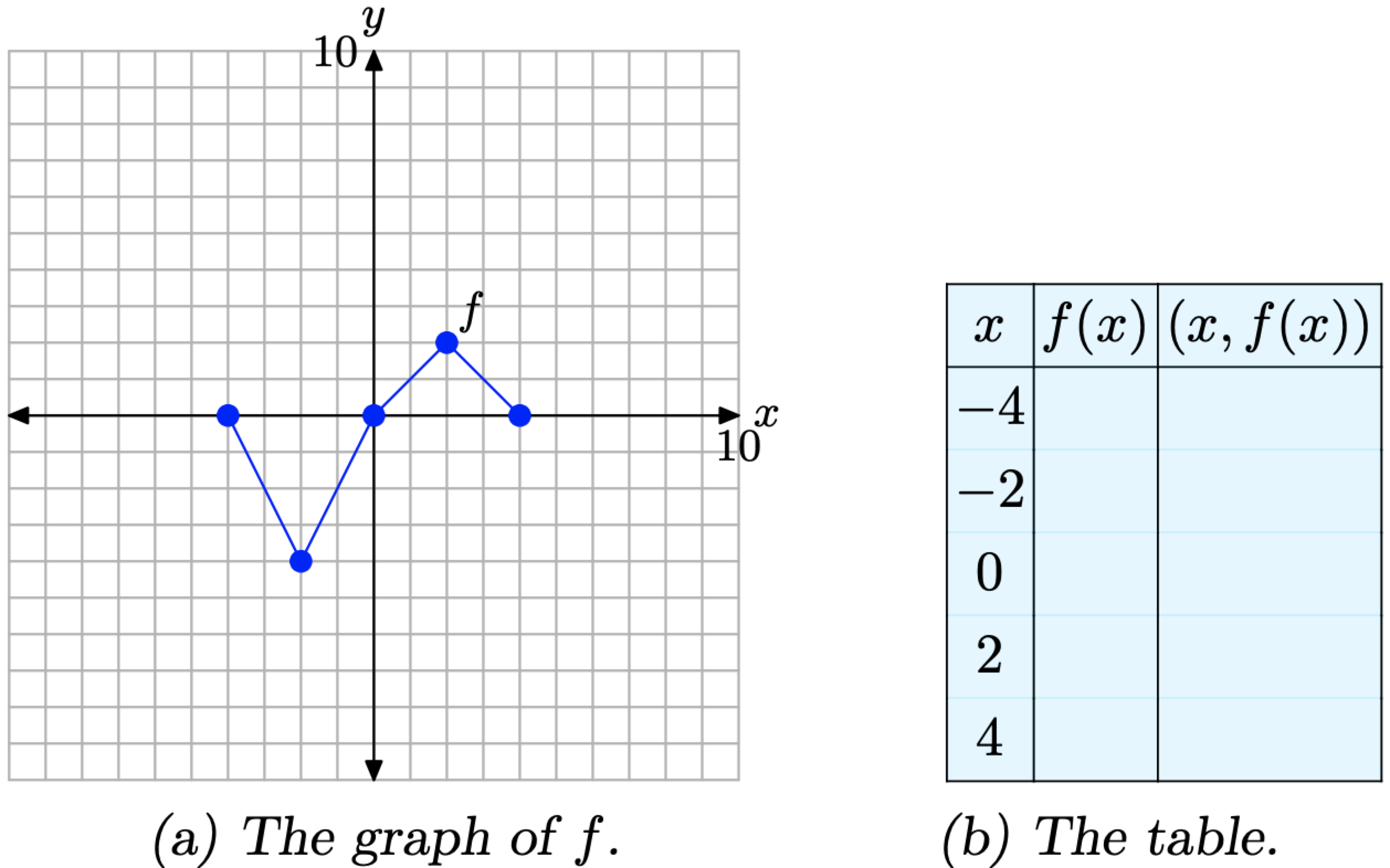
Figure \(\PageIndex{1}\). Reading key values from the graph of f.

Solution

To compute f(−2), for example, we would first locate −2 on the x-axis, draw a vertical arrow to the graph of f, then a horizontal arrow to the y-axis, as shown in Figure \(\PageIndex{2}\)(a). The y-value of this final destination is the value of f(−2). That is, f(−2) = −4. This allows us to complete one entry in the table, as shown in Figure \(\PageIndex{2}\)(b). Continue in this manner to complete all of the entries in the table. The result is shown in Figure \(\PageIndex{2}\)(c).

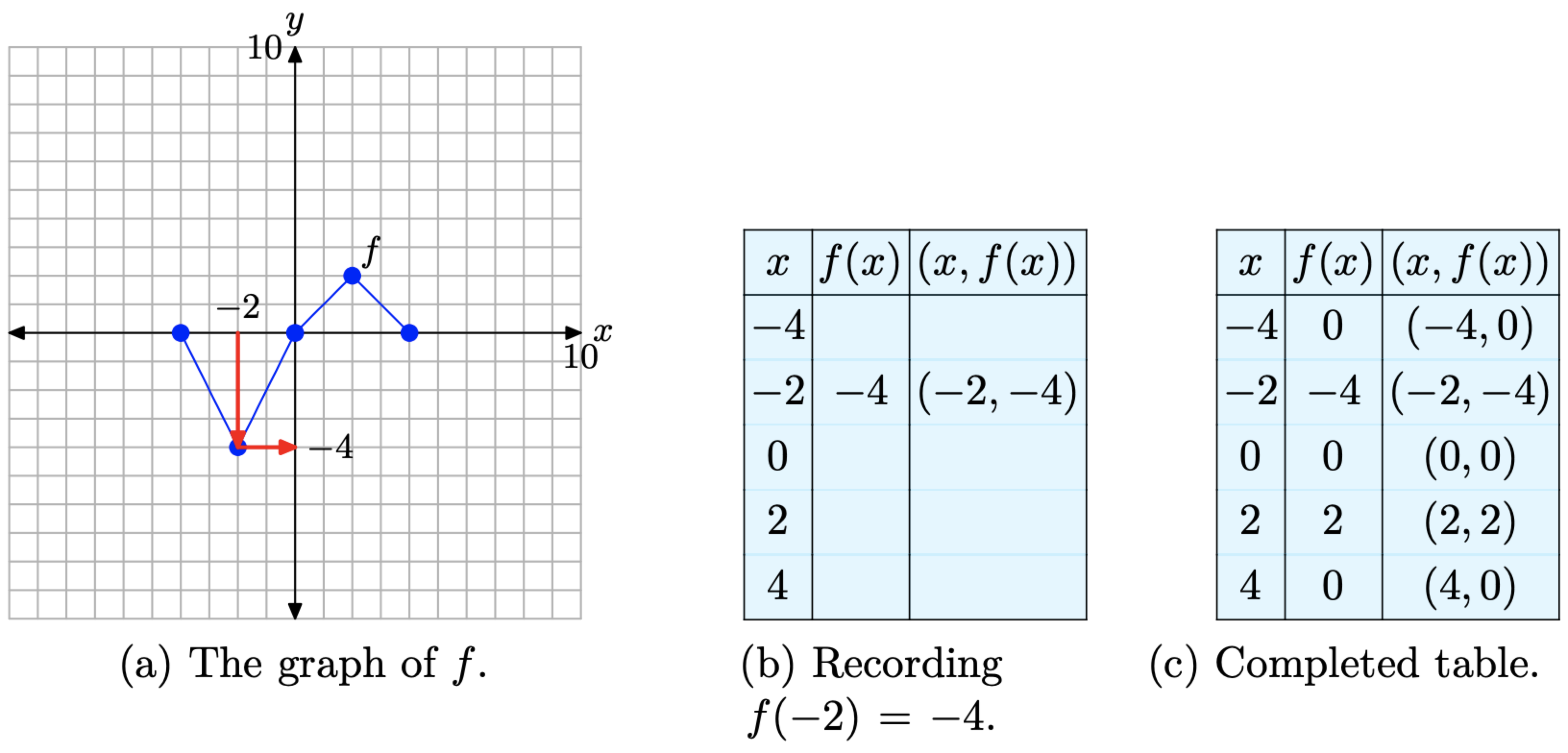
Figure \(\PageIndex{2}\). Recording coordinates of points on the graph of f in the tables

Horizontal Scaling

In the narrative that follows, we will have repeated need of the graph in Figure \(\PageIndex{2}\)(a) and the table in Figure \(\PageIndex{2}\)(c). They characterize the basic function that will be the starting point for the concepts of scaling, reflection, and translation that we develop in this section. Consequently, let’s place them side-by-side for emphasis in Figure \(\PageIndex{3}\).

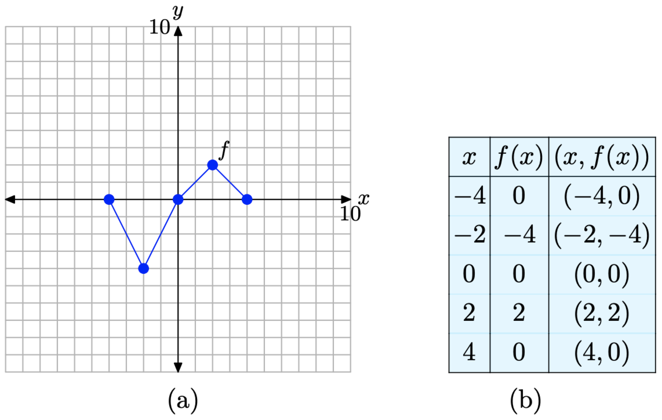
Figure \(\PageIndex{3}\). The original graph of f and a table of key points on the graph of f

We are now going to scale the graph of f in the horizontal direction.

Example \(\PageIndex{2}\)

If y = f(x) has the graph shown in Figure \(\PageIndex{3}\)(a), sketch the graph of y = f(2x).

Solution

In the previous section, we investigated the graph of y = 2f(x). The number 2 was outside the function notation and as a result we stretched the graph of y = f(x) vertically by a factor of 2. However, note that the 2 is now inside the function notation y = f(2x). Intuition would demand that this might have something to do with scaling in the x-direction (horizontal direction), but how?

Again, when we’re unsure of the shape of the graph, we rely on plotting a table of points. We begin by picking these x-values: x = −2, −1, 0, 1, and 2. Note that these are precisely half of each of the x-values presented in the table in Figure \(\PageIndex{3}\)(b). We will now evaluate the function y = f(2x) at each of these x-values. For example, to compute y = f(2x) at x = −2, we first insert x = −2 for x to obtain \[y=f(2(-2))=f(-4) \nonumber \]

To complete the computation, we must now evaluate f(−4). However, this result is recorded in the table in Figure \(\PageIndex{3}\)(b). There we find that f(−4) = 0, and we can complete the computation started above.

\[y=f(2(-2))=f(-4)=0 \nonumber \]

In similar fashion, to evaluate the function y = f(2x) at x = −1, first substitute x = −1 in y = f(2x) to obtain

\[y=f(2(-1))=f(-2) \nonumber \]

Now, note that f(−2) is the next recorded value in the table in Figure \(\PageIndex{3}\)(b). There we find that f(−2) = −4, so we can complete the computation started above.

\[y=f(2(-1))=f(-2)=-4 \nonumber \]

At this point, you might see why we chose x-values: −2, −1, 0, 1, and 2. These are precisely half of the x-values in the table of original values for the function y = f(x) in Figure \(\PageIndex{3}\)(b). When the values −2, −1, 0, 1, and 2 are substituted into the function y = f(2x), they are first doubled before we go to look up the function value in the table in Figure \(\PageIndex{3}\)(b).

Continuing in this manner, we evaluate the function y = f(2x) at the remaining values of x, namely, 0, 1, and 2.

\[\begin{aligned} y &=f(2(0))=f(0)=0 \\ y &=f(2(1))=f(2)=2 \\ y &=f(2(2))=f(4)=0 \end{aligned} \nonumber \]

We enter these values into the table in Figure 4(b) and plot them to determine the graph of y = f(2x) in Figure \(\PageIndex{4}\)(a).

At this point, there are a number of comparisons you can make.

1. Compare the data in the table in Figure \(\PageIndex{4}\)(b) with the original function data in the table in Figure \(\PageIndex{3}\)(b). Note that the y-values in each table are identical. However, note that each x-value in the table of Figure \(\PageIndex{4}\)(b) is precisely half of the corresponding x-value in the table of Figure \(\PageIndex{3}\)(b).

2. Compare the graph of y = f(2x) in Figure \(\PageIndex{4}\)(a) with the original graph of y = f(x) in Figure \(\PageIndex{3}\)(a). Note that each x-value at each point on the graph of y = f(2x) in

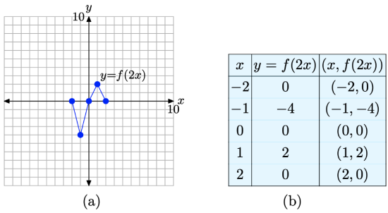
Figure \(\PageIndex{4}\). The points in the table are points on the graph of y = f(2x).

Figure \(\PageIndex{4}\)(a) is precisely half the x-value of the corresponding point on the graph of y = f(x) in Figure \(\PageIndex{3}\)(a).

Note the result. The graph of y = f(2x) is compressed horizontally (toward the y-axis), both positively and negatively, by a factor of 2. Note that this is exactly the opposite of what you might expect by intuition, but a careful examination of the data in the tables in Figures \(\PageIndex{3}\)(b) and \(\PageIndex{4}\)(b) will explain why.

Let’s look at another example.

Example \(\PageIndex{3}\)

If y = f(x) has the graph shown in Figure \(\PageIndex{3}\)(a), sketch the graph of y = f((1/2)x).

Solution

Rather than doubling each value of x at the start, this function first halves each value of x. Thus, we will want to evaluate the function y = f((1/2)x) at x = −8, −4, 0, 4, and 8. For example, to evaluate the function y = f((1/2)x) at x = −8, first substitute x = −8 to obtain \[y=f((1 / 2)(-8))=f(-4) \nonumber \]

Now, look up this value in the table in Figure \(\PageIndex{3}\)(b) and note that f(−4) = 0. Thus, we can complete the computation as follows.

\[y=f((1 / 2)(-8))=f(-4)=0 \nonumber \]

Similarly, to evaluate the function y = f((1/2)x) at x = −4, first substitute x = −4 to obtain

\[y=f((1 / 2)(-4))=f(-2) \nonumber \]

Now, look up this value in the table in Figure \(\PageIndex{3}\)(b) and note that f(−2) = −4. Thus, we can complete the computation as follows.

\[y=f((1 / 2)(-4))=f(-2)=-4 \nonumber \]

At this point, you will see why we chose x-values: −8, −4, 0, 4, and 8. These values are precisely double the x-values in the table of original values for the function y = f(x) in Figure \(\PageIndex{3}\)(b). When the values −8, −4, 0, 4, and 8 are substituted into the function y = f((1/2)x), they are first halved before we go to look up the function value in the table in Figure \(\PageIndex{3}\)(b). This halving leads to the values −4, −2, 0, 2, and 4, which are precisely the values available in the table in Figure \(\PageIndex{3}\)(b).

We make similar computations at the remaining values of x, namely x = 0, 4, and 8.

\[\begin{aligned} y &=f((1 / 2)(0))=f(0)=0 \\ y &=f((1 / 2)(4))=f(2)=2 \\ y &=f((1 / 2)(8))=f(4)=0 \end{aligned} \nonumber \]

Hopefully, these computations explain our choice of x-values above. Each of these results is recorded in the table in Figure \(\PageIndex{5}\)(b) and plotted on the graph shown in Figure \(\PageIndex{5}\)(a).

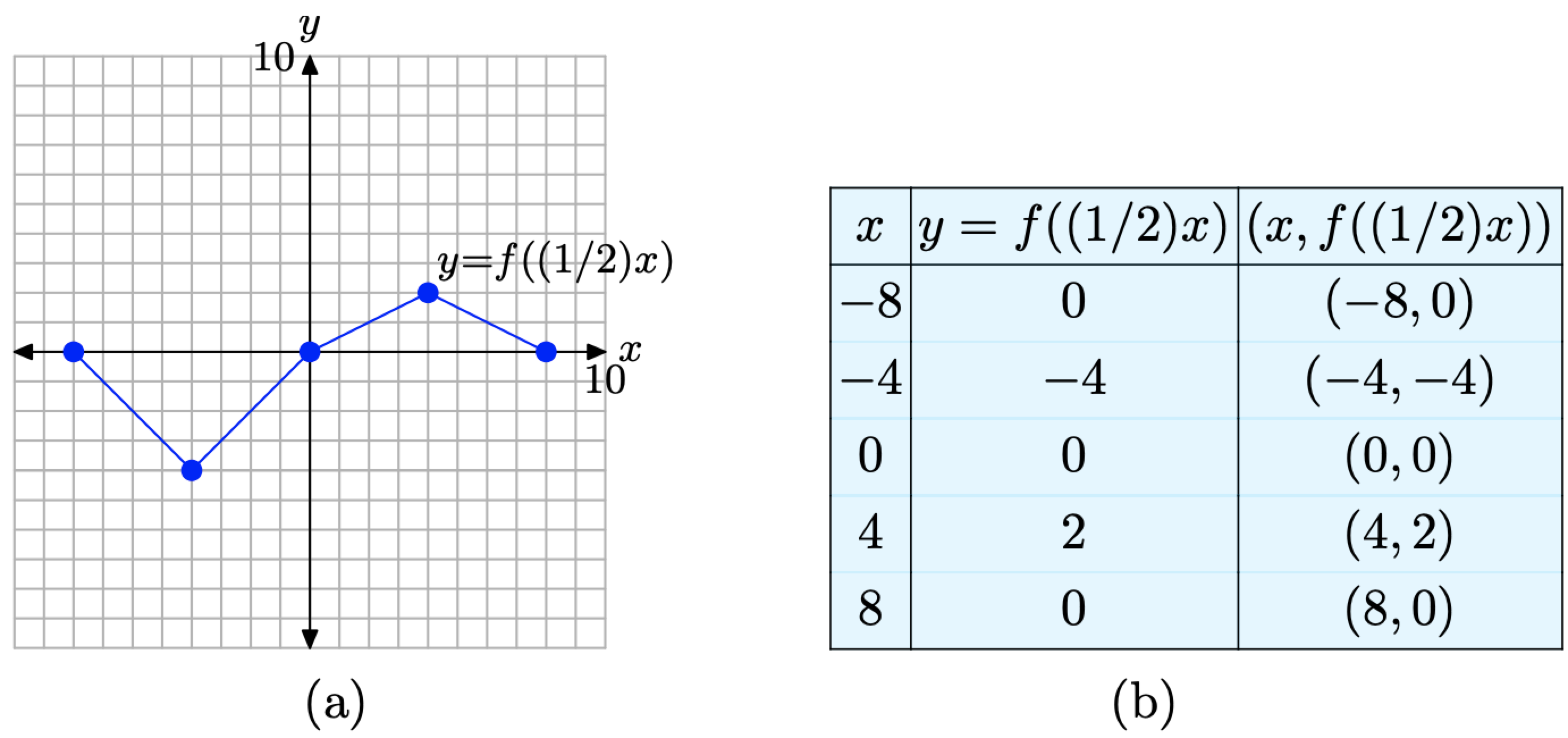
Figure \(\PageIndex{5}\). The points in the table are points on the graph of y = f((1/2)x).

Again, note that the y-values in the table in Figure \(\PageIndex{5}\)(b) are identical to the y-values in the table in Figure \(\PageIndex{3}\)(b). However, each x-value in the table in Figure \(\PageIndex{5}\)(b) is precisely double the corresponding x-value in the table in Figure \(\PageIndex{3}\)(b).

This doubling of the x-values is apparent in the graph of y = f((1/2)x) shown in Figure \(\PageIndex{5}\)(a), where the graph is stretched by a factor of 2 horizontally (away from the y-axis), both positively and negatively. Note that this is exactly the opposite of what you might expect by intuition, but a careful examination of the data in the tables in Figures \(\PageIndex{3}\)(b) and \(\PageIndex{5}\)(b) will explain why.

Let’s summarize our findings.

A Visual Summary — Horizontal Scaling

Consider the images in Figure \(\PageIndex{6}\).

• In Figure \(\PageIndex{6}\)(a), we see pictured the graph of the original function y = f(x).
• In Figure \(\PageIndex{6}\)(b), note that each key point on the graph of y = f(2x) has an x-value that is precisely half the x-value of the corresponding point on the graph of y = f(x) in Figure \(\PageIndex{6}\)(a).
• In Figure \(\PageIndex{6}\)(c), note that each key point on the graph of y = f((1/2)x) has an x-value that is twice the x-value of the corresponding point on the graph of y = f(x) in Figure \(\PageIndex{6}\)(a).
• Note that the y-value of each transformed point remains the same.

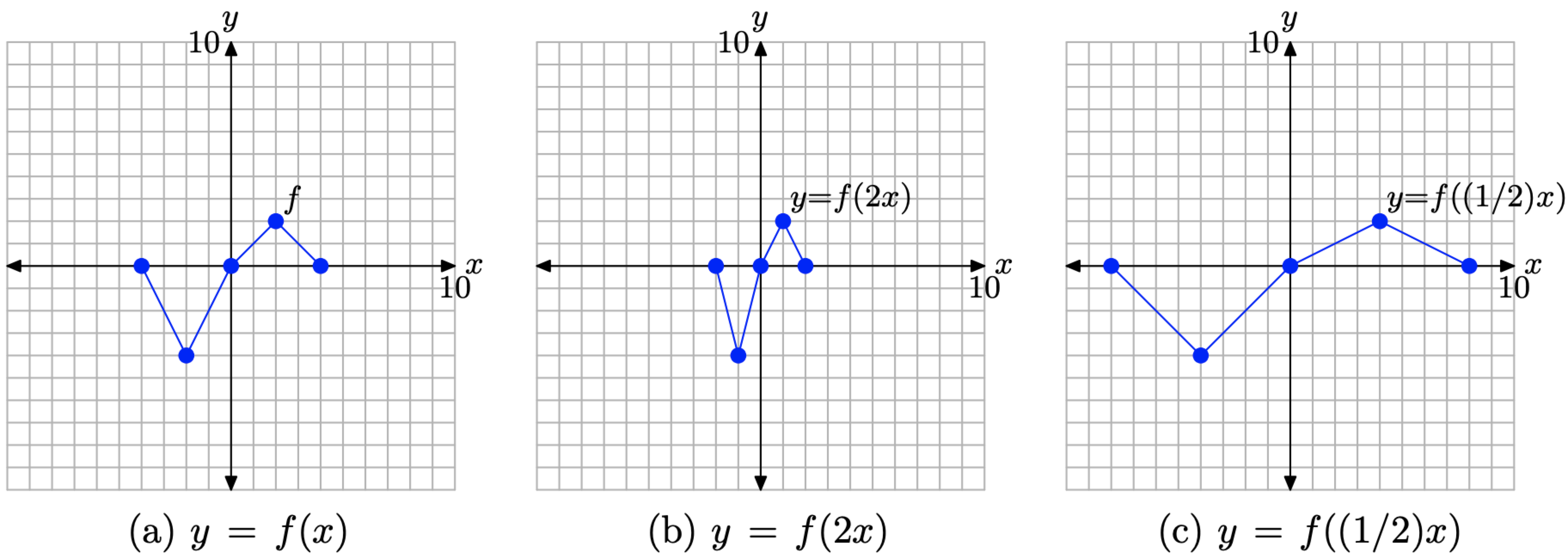
Figure \(\PageIndex{6}\). The graph of y = f(2x) compresses horizontally (toward the y-axis) by a factor of 2. The graph of y = f((1/2)x) stretches horizontally (away from the y-axis) by a factor of 2.

The visual summary in Figure \(\PageIndex{6}\) makes sketching the graphs of y = f(2x) and y = f(1/2)x) an easy task.

• Given the graph of y = f(x), to sketch the graph of y = f(2x), simply take each point on the graph of y = f(x) and cut its x-value in half, keeping the same y-value.
• Given the graph of y = f(x), to sketch the graph of y = f((1/2)x), simply take each point on the graph of y = f(x) and double its x-value, keeping the same y-value.

Follow the same procedures for other scaling factors. For example, in the case of y = f(3x), take each point on the graph of y = f(x) and divide its x-value by 3, keeping the same y-value. On the other hand, to draw the graph of y = f((1/3)x), take each point on the graph of f and multiply its x-value by 3, keeping the same y-value.

In general, we can state the following.

summary

Suppose we are given the graph of y = f(x).

• If a > 1, the graph of y = f(ax) compresses horizontally (toward the y-axis) , both positively and negatively, by a factor of a.
• If 0 < a < 1, the graph of y = f(ax) stretches horizontally (away from the y-axis), both positively and negatively, by a factor of 1/a.

In the case of the first item in Summary, when we compare the general form y = f(ax) with y = f(2x), we see that a = 2. In this case, note that a > 1 and the graph of y = f(2x) compresses horizontally by a factor of 2 when compared with the graph of y = f(x) (see Figure \(\PageIndex{6}\)(b)).

In the case of the second item in Summary, when we compare the general form y = f(ax) with the equation y = f((1/2)x), we see that a = 1/2, so

\[\frac{1}{a}=\frac{1}{1 / 2}=2 \nonumber \]

The second item in Summary 4 says that when 0 < a < 1, the graph of y = f(ax) stretches horizontally by a factor of 1/a. Indeed, this is exactly what happened in the case of y = f((1/2)x), which stretched in the horizontal direction by a factor of 1/(1/2), or 2 (see Figure \(\PageIndex{6}\)(c)).

Horizontal Reflections

For convenience, we begin by repeating the original graph of y = f(x) and its accompanying data in Figure \(\PageIndex{7}\). We are now going to reflect the graph of y = f(x) in the horizontal direction (across the y-axis).

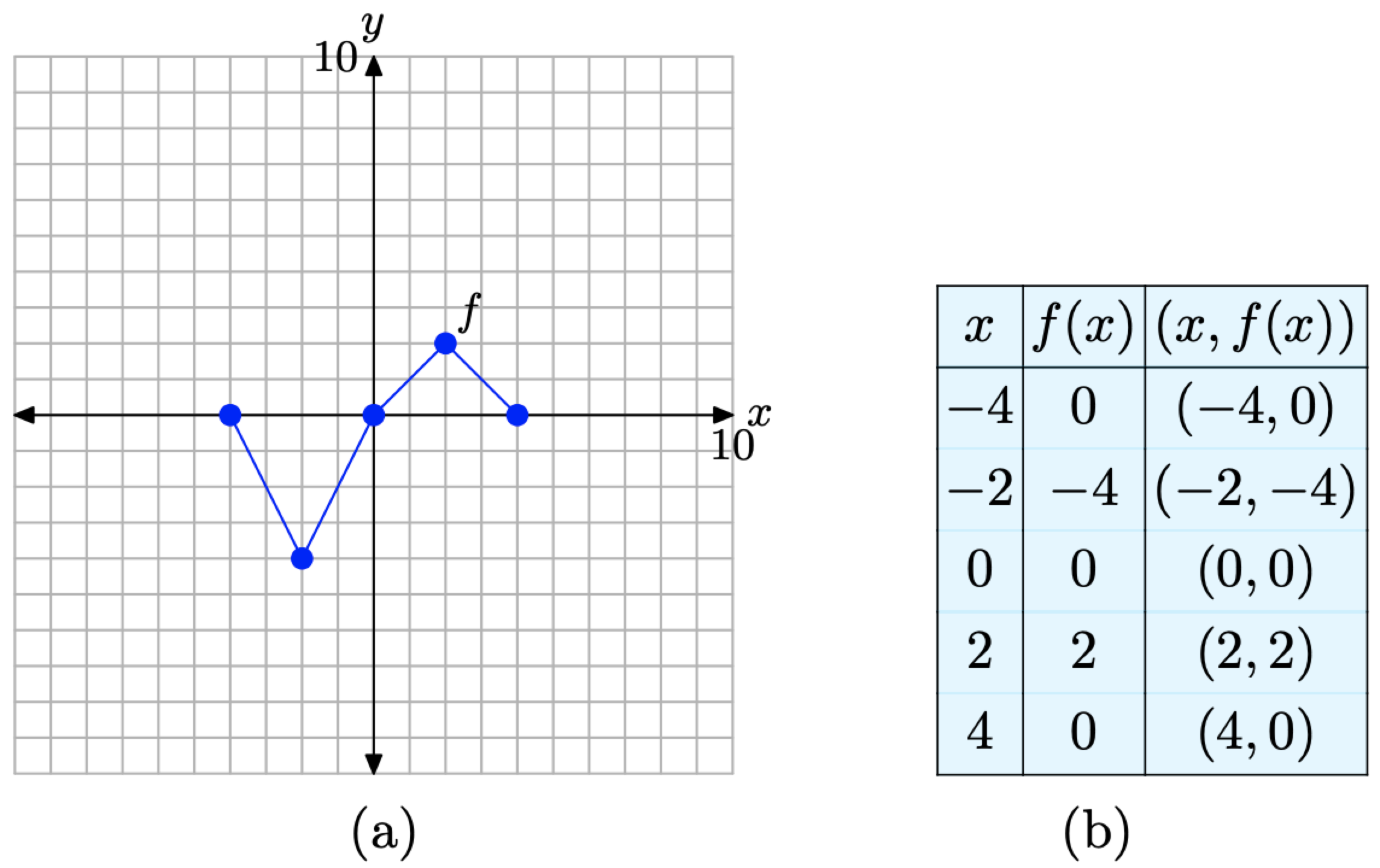
Figure \(\PageIndex{7}\). The original graph of f and a table of key points on the graph of f

Example \(\PageIndex{4}\)

If y = f(x) has the graph shown in Figure \(\PageIndex{7}\)(a), draw the graph of y = f(−x).

Solution

In the previous section, we were asked to draw the graph of y = −f(x). Note how the minus sign appears on the outside of the function. Clearly, the y-values of y = −f(x) must be opposite in sign to the y-values of y = f(x). That is why the graph of y = −f(x) was a reflection of the graph of y = f(x) across the x-axis.

However, in this example, the minus sign is inside the function, leaving one to intuit that it is the x-values, not the y-values, that are being negated. We will choose the following x-values: x = 4, 2, 0, −2, and −4. This is a bit deceptive, as it looks like we are choosing the same x-values, only in reverse order. This is not the case. We are choosing the negative of each x-value in the table in Figure \(\PageIndex{7}\)(b).

To evaluate y = f(−x) at our first x-value, namely x = 4, we perform the following calculation. First substitute x = 4 to obtain

\[y=f(-(4))=f(-4) \nonumber \]

Now, look up this value in the table in Figure \(\PageIndex{7}\)(b) and note that f(−4) = 0. Thus, we can complete the computation as follows.

\[y=f(-(4))=f(-4)=0 \nonumber \]

Similarly, to evaluate the function y = f(−x) at x = 2, first substitute x = 2 to obtain

\[y=f(-(2))=f(-2) \nonumber \]

Now, look up this value in the table in Figure \(\PageIndex{7}\)(b) and note that f(−2) = −4. Thus, we can complete the computation as follows.

\[y=f(-(2))=f(-2)=-4 \nonumber \]

At this point, you will see why we chose x-values: 4, 2, 0, −2, and −4. These values are the negatives of the x-values in the table of original values for the function y = f(x) in Figure \(\PageIndex{7}\)(b). When the values 4, 2, 0, −2, and −4 are substituted into the function y = f(−x), they are first negated before we go to look up the function value in the table in Figure \(\PageIndex{7}\)(b). This negating leads to the values −4, −2, 0, 2, and 4, which are precisely the values available in the table in Figure \(\PageIndex{7}\)(b).

We make similar computations at the remaining values of x, namely x = 0, −2, and −4.

\[\begin{array}{l}{y=f(-(0))=f(0)=0} \\ {y=f(-(-2))=f(2)=2} \\ {y=f(-(-4))=f(4)=0}\end{array} \nonumber \]

We organize these points in the table in Figure \(\PageIndex{8}\)(b), then plot them in Figure \(\PageIndex{8}\)(a).

When you compare the entries in the table in Figure \(\PageIndex{8}\)(b) with those in the table in Figure \(\PageIndex{7}\)(b), note that the y-values appear in the same order, but the x-values of the table in Figure \(\PageIndex{7}\)(b) have been negated in the table in Figure \(\PageIndex{8}\)(b). This means that a former point such as (−2, −4) is transformed to the point (2, −4), which is a reflection of the point (−2, −4) across the y-axis.

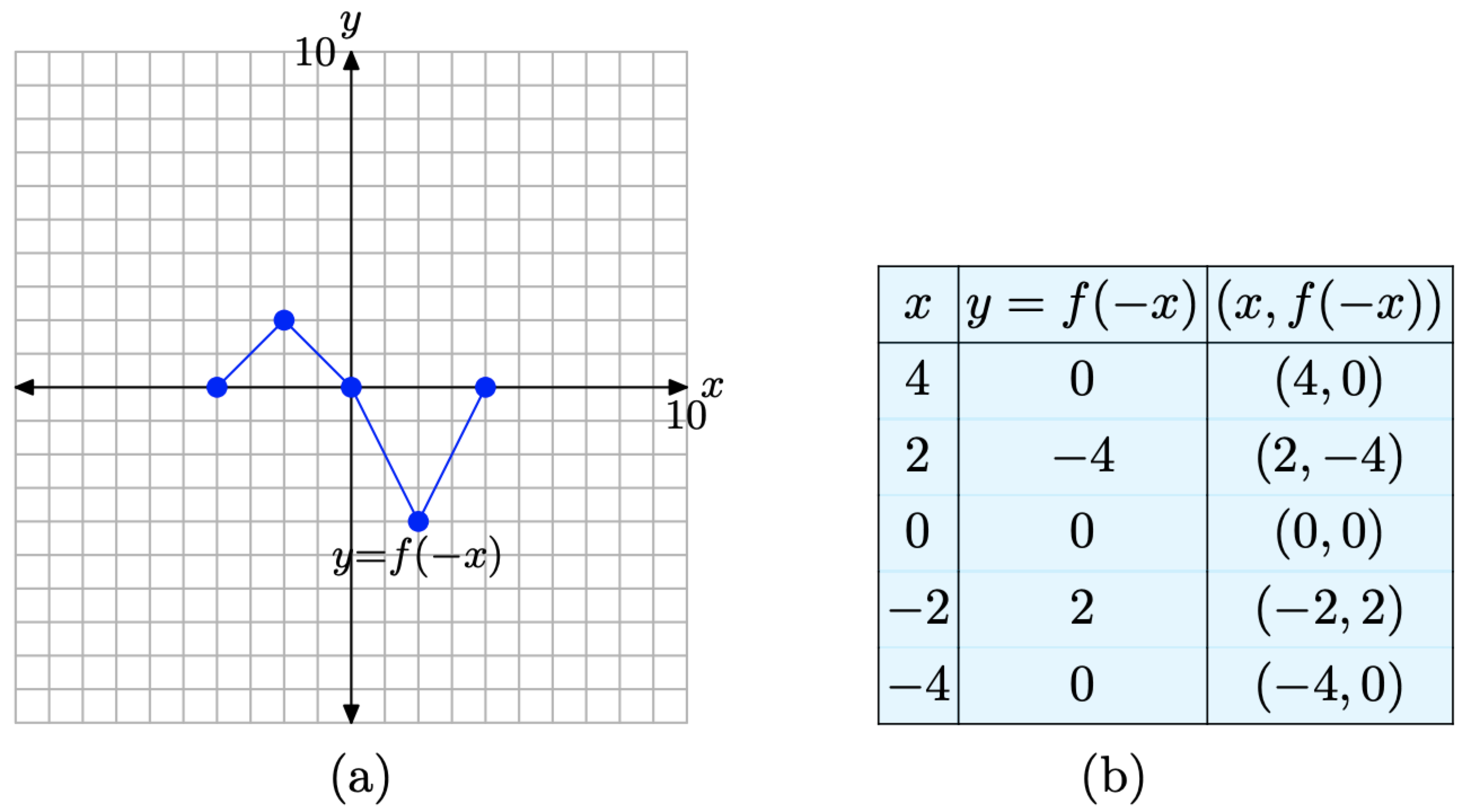
Figure \(\PageIndex{8}\). The graph of y = f(−x) and a table of key points on the graph.

Thus, to produce the graph of y = f(−x), simply reflect the graph of y = f(x) across the y-axis.

Let’s summarize what we’ve learned about horizontal reflections.

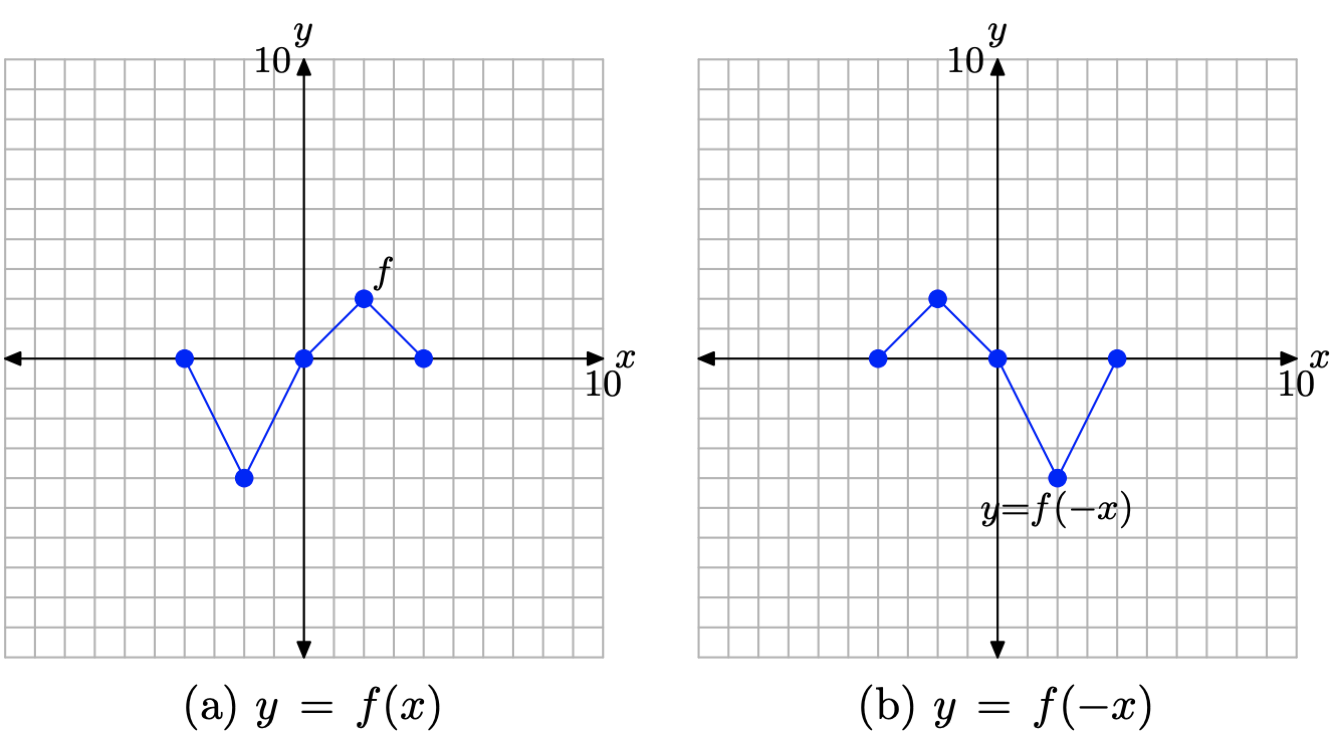
Figure \(\PageIndex{9}\). The graph of y = f(−x) is a reflection of the graph of y = f(x) across the y-axis.

A Visual Summary — Horizontal Reflections

Consider the images in Figure \(\PageIndex{9}\).

• In Figure \(\PageIndex{9}\)(a), we see pictured the original graph of y = f(x).
• In Figure \(\PageIndex{9}\)(b), the graph of y = f(−x) is a reflection of the graph of y = f(x) across the y-axis.

Thus, given the graph of y = f(x), it is a simple task to draw the graph of y = f(−x).

• To draw the graph of y = f(−x), take each point on the graph of y = f(x) and reflect it across the y-axis, keeping the y-value the same, but negating the x-value.

Horizontal Translations

In the previous section, we saw that the graphs of y = f(x) + c and y = f(x) − c were vertical translations of the graph of y = f(x). If c is a positive number, then the graph of y = f(x) + c shifts c units upward while the graph of y = f(x) − c shifts c units downward.

In this section, we will study horizontal translations. For convenience, we begin by repeating the original graph of y = f(x) and its accompanying data in Figure 10.

Figure \(\PageIndex{10}\). The original graph of f and a table of key points on the graph of f

Example \(\PageIndex{5}\)

If y = f(x) has the graph shown in Figure \(\PageIndex{10}\)(a), sketch the graph of y = f(x + 1).

Solution

In the previous section, we drew the graph of y = f(x)+1. Note that in y = f(x)+1, the number 1 is outside the function. The result was a graph that was shifted 1 unit upwards in the y-direction.

In this case, y = f(x + 1) and the 1 is inside the function notation, leading one to intuit that the translation might be in the horizontal direction (x-direction). But how?

Again, we will set up a table of points that satisfy the equation y = f(x + 1), then plot them. Because this function requires that we first add 1 to each x-value before inserting it into the function, we will choose x-values appropriately, namely x = −5, −3, −1, 1, and 3. In a moment, it will be clear why we have chosen these particular values of x. Perhaps you already see why?

We need to evaluate the function y = f(x + 1) at each of these chosen values of x. To evaluate y = f(x+ 1) at the first value, namely x = −5, we insert x = −5 and make the calculation \[y=f(-5+1)=f(-4) \nonumber \]

To complete the calculation, we must now evaluate f(−4). However, this result is recorded in the table in Figure \(\PageIndex{10}\)(b). There we find that f(−4) = 0, and we can complete the calculation started above.

\[y=f(-5+1)=f(-4)=0 \nonumber \]

In similar fashion, we can evaluate the function y = f(x+1) at x = −3. First, substitute x = −3 in y = f(x + 1) to obtain

\[y=f(-3+1)=f(-2) \nonumber \]

To complete the calculation, we must now evaluate f(−2). However, this result is recorded in the table in Figure \(\PageIndex{10}\)(b). There we find that f(−2) = −4, and we can complete the calculation started above.

\[y=f(-3+1)=f(-2)=-4 \nonumber \]

At this point, you might see why we chose x-values: −5, −3, −1, 1, and 3. These are precisely one less than the x-values in the table of original values for the function y = f(x) in Figure \(\PageIndex{10}\)(b). When the values −5, −3, −1, 1, and 3 are substituted into the function y = f(x + 1), we first add 1 to each value before we go to look up the function value in the table in Figure \(\PageIndex{10}\)(b). This adding of 1 leads to the values −4, −2, 0, 2, and 4, which are precisely the values available in the table in Figure \(\PageIndex{10}\)(b).

Continuing in this manner, we evaluate the function y = f(x + 1) at the remaining values of x, namely, −1, 1, and 3.

\[\begin{aligned} y &=f(-1+1)=f(0)=0 \\ y &=f(1+1)=f(2)=2 \\ y &=f(3+1)=f(4)=0 \end{aligned} \nonumber \]

We assemble these results in the table in Figure \(\PageIndex{11}\)(b) and plot them in Figure \(\PageIndex{11}\)(a).

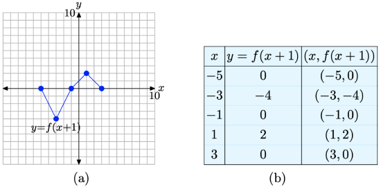
Figure \(\PageIndex{11}\). The graph of y = f(x + 1) and a table of key points on the graph

When you compare the points on the graph of y = f(x+1) in the table in Figure \(\PageIndex{11}\)(b) with the original points on the graph of y = f(x) in the table in Figure \(\PageIndex{10}\)(b), note that the y-values are identical, but the x-values in the table in Figure \(\PageIndex{11}\)(b) are all 1 unit less than the corresponding x-values in the table in Figure \(\PageIndex{10}\)(b). It is no wonder that the graph of y = f(x + 1) in Figure \(\PageIndex{11}\)(a) is shifted 1 unit to the left of the original graph of y = f(x) in Figure \(\PageIndex{10}\)(a).

Note that this is somewhat counterintuitive, because we’re seemingly adding 1 to each x-value in y = f(x + 1). Why doesn’t the graph move one unit to the right? Well, a careful comparison of the x-values in the tables in Figures \(\PageIndex{10}\)(b) and \(\PageIndex{11}\)(b) reveals the answer. In order to use the data in the table in Figure \(\PageIndex{10}\)(b), we must first subtract 1 from each x-value to produce the x-values in the table in Figure \(\PageIndex{11}\)(b). This is why the graph of y = f(x + 1) moves 1 unit to the left instead of 1 unit to the right.

You might also recall that the function y = f(2x) compressed by a factor of 2, which is also the opposite of what intuition might dictate. Similarly, the function y = f((1/2)x) stretches by a factor of 2, which also goes counter to intuition. With these thoughts in mind, it is not surprising that y = f(x+ 1) shifts one unit to the left. Still, a comparison of the x-values in the tables in Figures \(\PageIndex{10}\)(b) and \(\PageIndex{11}\)(b) provide irrefutable evidence that the shift is 1 unit to the left.

Let’s look at another example.

Example \(\PageIndex{6}\)

If y = f(x) has the graph shown in Figure \(\PageIndex{10}\)(a), sketch the graph of y = f(x − 2).

Solution

Again, we will set up a table of points that satisfy the equation y = f(x − 2), then plot them. Because this function requires that we first subtract 2 from each x-value before inserting it into the function, we will choose x-values: −2, 0, 2, 4, and 6. We need to evaluate the function y = f(x − 2) at each of these values of x.

To evaluate y = f(x − 2) at the first value, namely x = −2, insert x = −2 into the function y = f(x − 2) to obtain \[y=f(-2-2)=f(-4) \nonumber \]

In the table in Figure \(\PageIndex{10}\)(b), we find that f(−4) = 0, which allows us to complete the calculation above.

\[y=f(-2-2)=f(-4)=0 \nonumber \]

In similar fashion, we evaluate y = f(x − 2) at x = 0 to obtain

\[y=f(0-2)=f(-2) \nonumber \]

In the table in Figure \(\PageIndex{10}\)(b), we find that f(−2) = −4, which allows us to complete the calculation above.

\[y=f(0-2)=f(-2)=-4 \nonumber \]

Hopefully, you see why we chose the x-values: −2, 0, 2, 4, and 6. These values are 2 larger than the x-values in the table of original values for the function y = f(x) in Figure \(\PageIndex{10}\)(b). When the values −2, 0, 2, 4, and 6 are substituted into the function y = f(x − 2), we first subtract 2 from each value before we go to look up the function value in the table in Figure \(\PageIndex{10}\)(b). This subtracting of 2 leads to −4, −2, 0, 2, and 4, precisely the values that are available in the table in Figure \(\PageIndex{10}\)(b).

Continuing in this manner, we evaluate y = f(x − 2) at the remaining values of x, namely, x = 2, 4, and 6.

\[\begin{array}{l}{y=f(2-2)=f(0)=0} \\ {y=f(4-2)=f(2)=2} \\ {y=f(6-2)=f(4)=0}\end{array} \nonumber \]

We assemble these results in the table in Figure \(\PageIndex{12}\)(b) and plot them in Figure \(\PageIndex{12}\)(a).

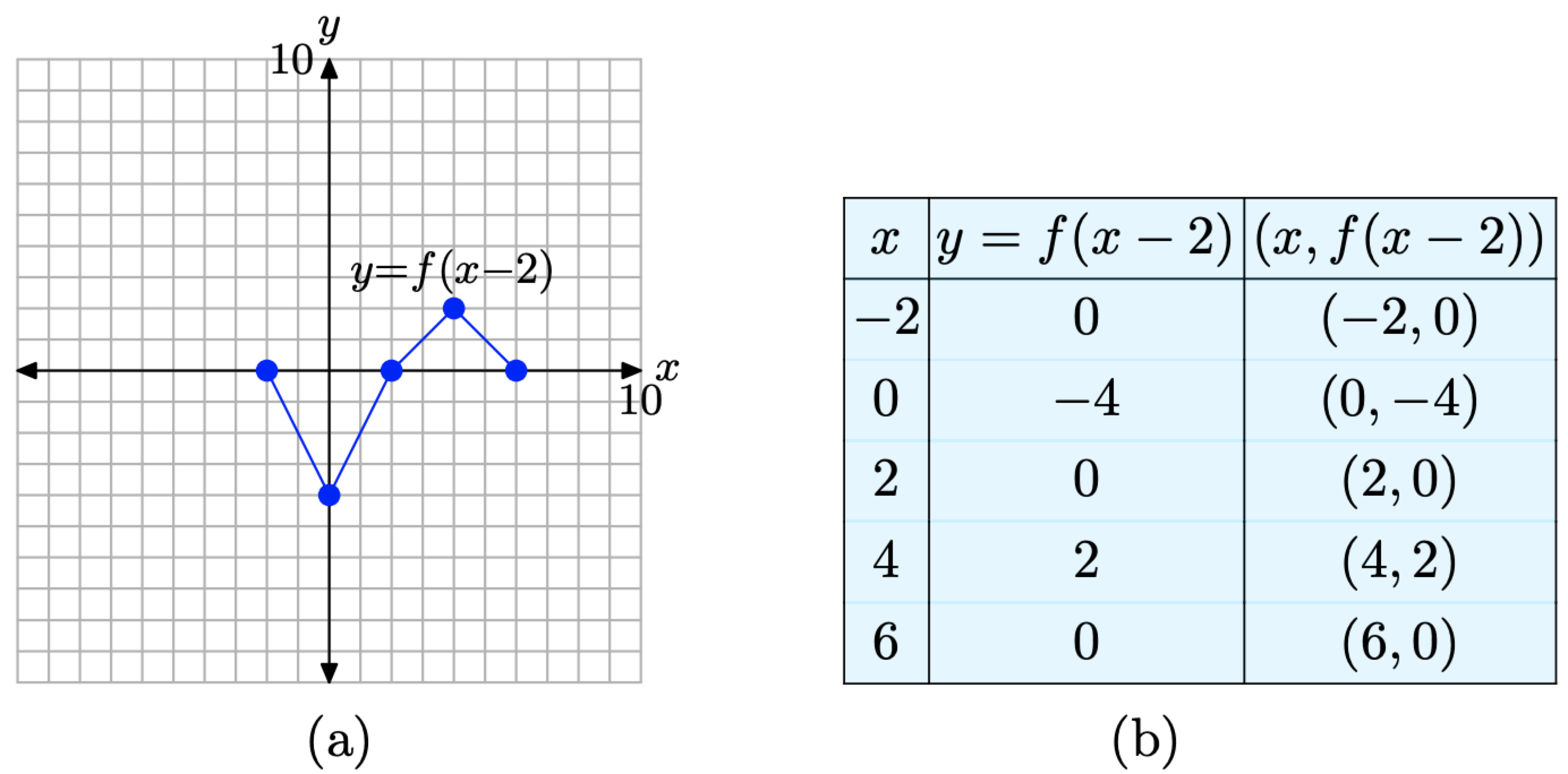
Figure \(\PageIndex{12}\). The graph of y = f(x − 2) and a table of key points on the graph.

When you compare the points on the graph of y = f(x−2) in the table in Figure \(\PageIndex{12}\)(b) with the original points on the graph of y = f(x) in the table in Figure \(\PageIndex{10}\)(b), note that the y-values are identical, but the x-values in the table in Figure \(\PageIndex{12}\)(b) are all 2 larger than the corresponding x-values in the table in Figure \(\PageIndex{10}\)(b). It is no wonder that the graph of y = f(x − 2) in Figure \(\PageIndex{12}\)(a) is shifted 2 units to the right of the original graph of y = f(x) in Figure \(\PageIndex{10}\)(a).

Again, this runs counterintuitive (why doesn’t the graph of y = f(x − 2) shift 2 units to the left?), but a comparison of the x-values in the tables in Figures \(\PageIndex{10}\)(b) and \(\PageIndex{12}\)(b) clearly indicates a shift to the right.

Let’s summarize what we’ve learned about horizontal translations.

Visual Summary — Horizontal Translations (Shifts)

Consider the images in Figure \(\PageIndex{13}\).

• In Figure \(\PageIndex{13}\)(a), we see pictured the graph of the original function y = f(x).
• In Figure \(\PageIndex{13}\)(b), note that each point on the graph of y = f(x + 1) has an x-value that is 1 unit less than the x-value of the corresponding point on the graph of y = f(x) in Figure \(\PageIndex{13}\)(a).
• In Figure \(\PageIndex{13}\)(c), note that each point on the graph of y = f(x − 2) has an x-value that is 2 units greater than the x-value of the corresponding point on the graph of y = f(x) in Figure \(\PageIndex{13}\)(a).
• Note that the y-value of each transformed point remains the same.

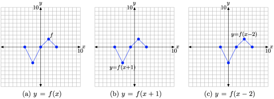
Figure \(\PageIndex{13}\). The graph of y = f(x + 1) is formed by shifting (horizontally) the graph of y = f(x) one unit to the left. The graph of y = f(x − 2) is formed by shifting (horizontally) the graph of y = f(x) two units to the right.

The visual summary in Figure \(\PageIndex{13}\) makes sketching the graphs of y = f(x + 1) and y = f(x − 2) an easy task.

• Given the graph of y = f(x), to sketch the graph of y = f(x + 1), simply take each point on the graph of y = f(x) and shift it 1 unit to the left, keeping the same y-value.
• Given the graph of y = f(x), to sketch the graph of y = f(x − 2), simply take each point on the graph of y = f(x) and shift it 2 units to the right, keeping the same y-value.

In general, we can state the following.

Summary

Suppose that we are given the graph of y = f(x) and suppose that c is any positive real number.

• The graph of y = f(x+c) is shifted c units to the left of the graph of y = f(x).
• The graph of y = f(x−c) is shifted c units to the right of the graph of y = f(x).

When we looked at vertical translations in the previous section, a translation was described by first imagining a graph on a sheet of transparent plastic, then sliding the transparency (without rotating it) over a coordinate system on a sheet of graph paper. Horizontal translations can be thought of in the same way, as sliding the graph on the transparency c units to the left, or c units to the right.

Extra Practice

In this section, let’s take the concepts from the Visual Summaries and put them to work on some final examples.

Example \(\PageIndex{7}\)

Consider the graph of f in Figure \(\PageIndex{14}\).

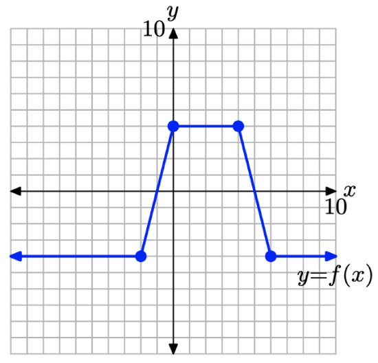
Figure \(\PageIndex{14}\). The graph of y = f(x) for Example \(\PageIndex{7}\).

Use the concepts from the Visual Summaries (scaling, reflection, and translation) to sketch the graphs of y = f(2x), y = f(−x), and y = f(x + 2) without creating and referring to tables.

Solution

To sketch the graph of y = f(2x), simply take each point on the graph of y = f(x) in Figure \(\PageIndex{15}\)(a) and divide its x-value by 2, keeping the same y-value. The result is shown in Figure \(\PageIndex{15}\)(b).

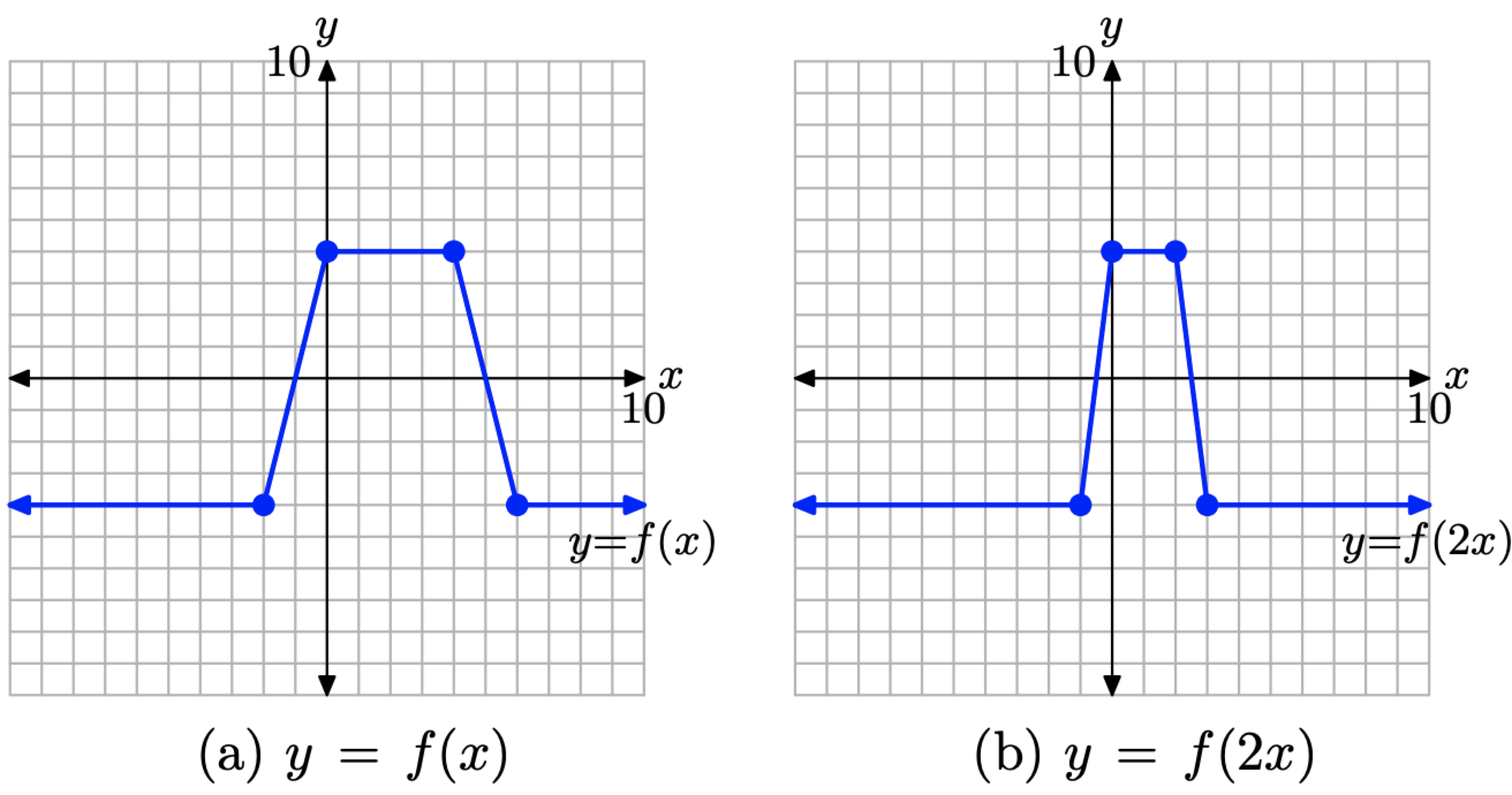
Figure \(\PageIndex{15}\). Compress the graph of y = f(x) by a factor of 2 to produce the graph of y = f(2x).

To sketch the graph of y = f(−x), simply take each point on the graph of y = f(x) in Figure \(\PageIndex{16}\)(a) and negate its x-value, keeping the same y-value. The result is shown in Figure \(\PageIndex{16}\)(b).

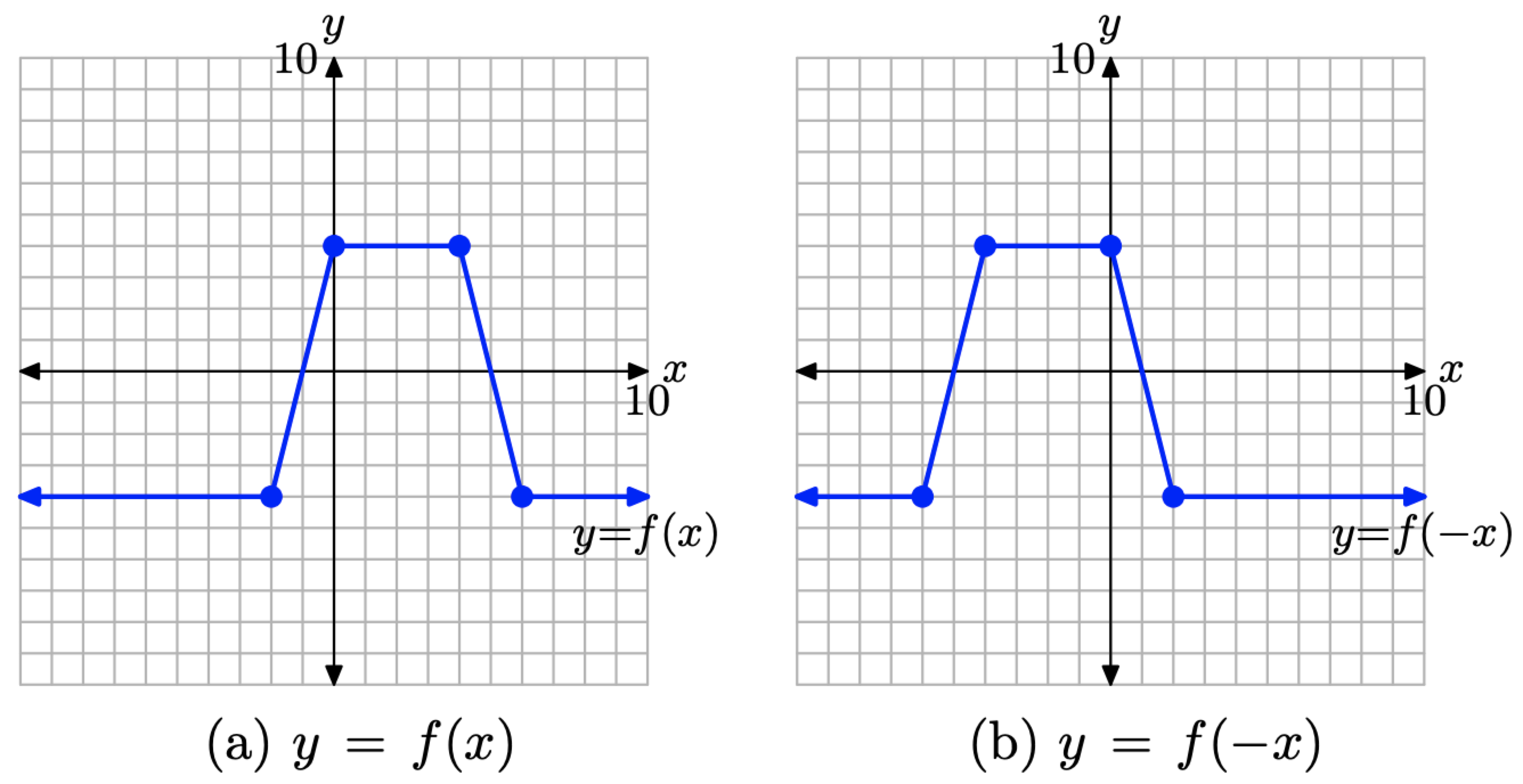
Figure \(\PageIndex{16}\). Reflect the graph of y = f(x) across the y-axis to produce the graph of y = f(−x).

To sketch the graph of y = f(x + 2), simply take each point on the graph of y = f(x) in Figure \(\PageIndex{17}\)(a) and subtract 2 from its x-value, keeping the same y-value. The result is shown in Figure \(\PageIndex{17}\)(b).

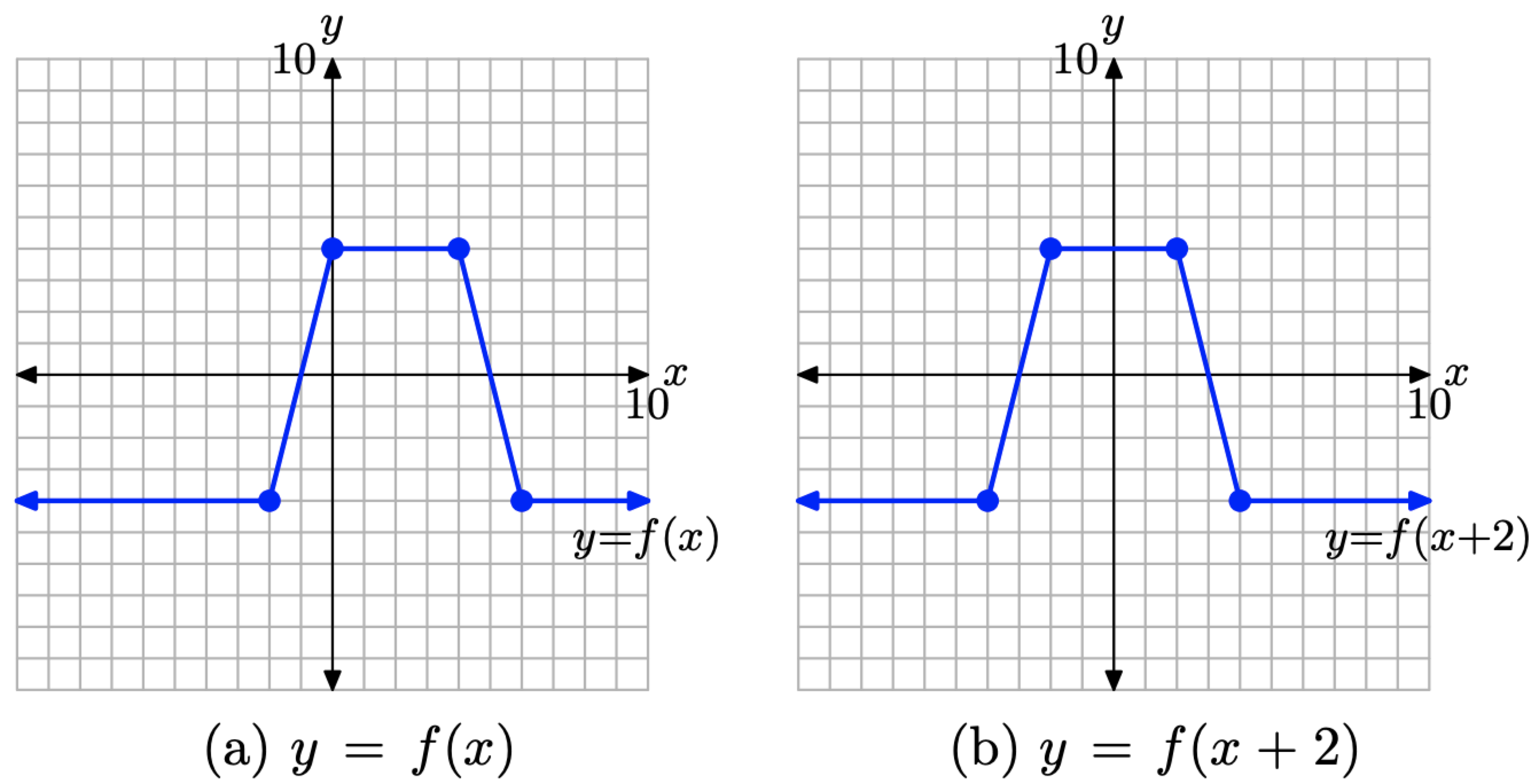
Figure \(\PageIndex{17}\). Shift the graph of y = f(x) to the left 2 units to produce the graph of y = f(x + 2).

Summary

In this section we’ve seen how a handful of transformations greatly enhance our graphing capability. We end this section by listing the transformations presented in this section and their effects on the graph of a function.

Vertical Transformations

Suppose we are given the graph of y = f(x).

• If a > 1, the graph of y = f(ax) compresses horizontally (toward the y-axis) , both positively and negatively, by a factor of a.
• If 0 < a < 1, the graph of y = f(ax) stretches horizontally (away from the y-axis), both positively and negatively, by a factor of 1/a.
• The graph of y = f(−x) is a reflection of the graph of y = f(x) across the y-axis.
• If c > 0, then the graph of y = f(x + c) is shifted c units to the left of the graph of y = f(x).
• If c > 0, then the graph of y = f(x − c) is shifted c units to the right of the graph of y = f(x).