2.5: Vertical Transformations

In this section we study the art of transformations: scalings, reflections, and translations. We will restrict our attention to transformations in the vertical or y-direction. Our goal is to apply certain transformations to the equation of a function, then ask what effect it has on the graph of the function.

We begin our task with an example that requires that we read the graph of a function to capture several key points that lie on the graph of the function.

Example \(\PageIndex{1}\)

Consider the graph of f presented in Figure \(\PageIndex{1}\)(a). Use the graph of f to complete the table in Figure \(\PageIndex{1}\)(b).

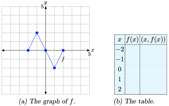
Figure \(\PageIndex{1}\). Reading key values from the graph of f.

Solution

To compute f(−1), we would locate −1 on the x-axis, draw a vertical arrow to the graph of f, then a horizontal arrow to the y-axis, as shown in Figure \(\PageIndex{2}\)(a). The y-value of this final destination is the value of f(−1). That is, f(−1) = 2. This allows us to complete one entry in the table, as shown in Figure \(\PageIndex{2}\)(b). Continue in this manner to complete all of the entries in the table. The result is shown in Figure \(\PageIndex{2}\)(c).

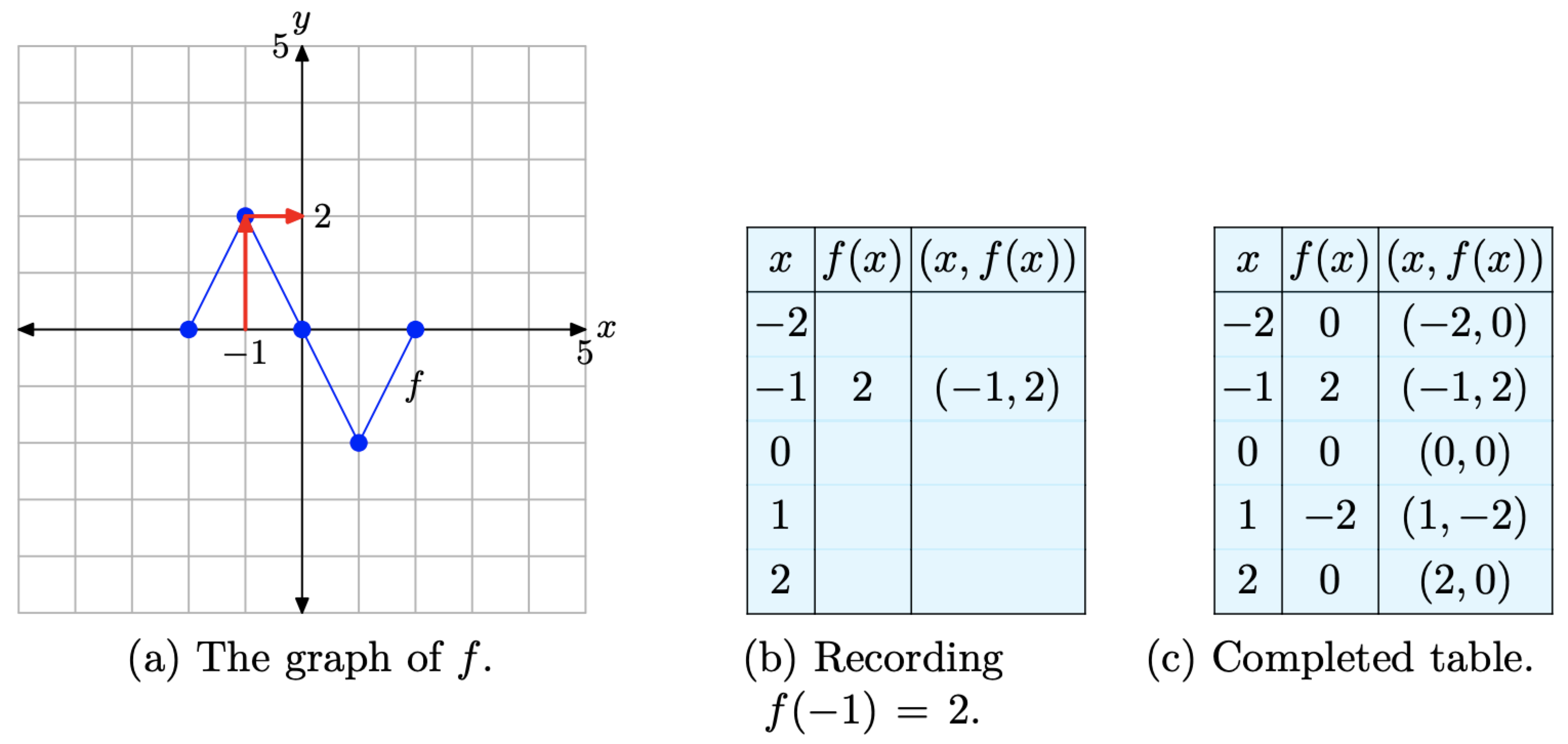
Figure \(\PageIndex{2}\). Recording coordinates of points on the graph of f in the tables.

Vertical Scaling

In the narrative that follows, we will have repeated need of the graph in Figure \(\PageIndex{2}\)(a) and the table in Figure \(\PageIndex{2}\)(c). They characterize the basic function that will be the starting point for the concepts of scaling, reflection, and translation that we develop in this section. Consequently, let’s place them side-by-side for emphasis in Figure \(\PageIndex{3}\).

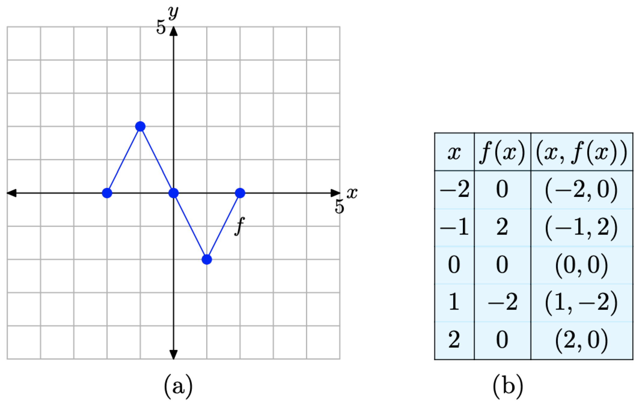
Figure \(\PageIndex{3}\). The original graph of f and a table of key points on the graph of f.

We are now going to scale the graph of f in the vertical direction.

Example \(\PageIndex{2}\)

If y = f(x) has the graph shown in Figure \(\PageIndex{3}\)(a), sketch the graph of y = 2f(x).

Solution

What do we do when we meet a graph whose shape we are unsure of? The answer to this question is we plot some points that satisfy the equation in order to get an idea of the shape of the graph. With that thought in mind, let’s evaluate the function y = 2f(x) at x = −2.

The letter f refers to the original function shown in Figure \(\PageIndex{3}\)(a) and the table in Figure \(\PageIndex{3}\)(b) contains the values of that function at the given values of x. Thus, in computing y = 2f(−2), the first step is to look up the value of f(−2) in the table in Figure \(\PageIndex{3}\)(b). There we find that f(−2) = 0. Thus, we can write \[y=2 f(-2)=2(0)=0 \nonumber \]

In similar fashion, let’s evaluate the function y = 2f(x) at x = −1. First, look up the value of f(−1) in the table in Figure \(\PageIndex{3}\)(b). There we find that f(−1) = 2. Thus, we can write \[y=2 f(-1)=2(2)=4 \nonumber \]

We finish by evaluating the function y = 2f(x) at x = 0, 1, and 2. Each time you need to evaluate the function f at a number, take the result from the table or graph in Figure 3. What follows are the evaluations of y = 2f(x) at x = −2, −1, 0, 1, and 2.

\[\begin{array}{l}{y=2 f(-2)=2(0)=0} \\ {y=2 f(-1)=2(2)=4} \\ {y=2 f(0)=2(0)=0} \\ {y=2 f(1)=2(-2)=-4} \\ {y=2 f(2)=2(0)=0}\end{array} \nonumber \]

We can arrange these results in a table shown in Figure \(\PageIndex{4}\)(b), then plot them in the figure shown in Figure \(\PageIndex{4}\)(a).

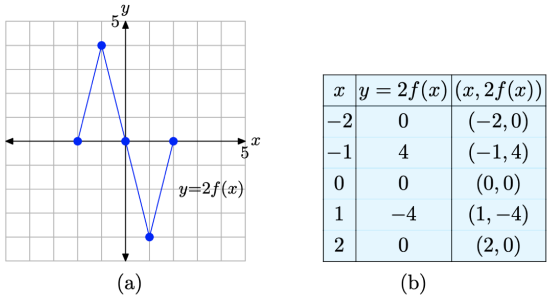
Figure \(\PageIndex{4}\). The points in the table are points on the graph of y = 2f(x).

At this point, there are a number of comparisons you can make.

1. Compare the data in the tables in Figure \(\PageIndex{3}\)(b) and Figure \(\PageIndex{4}\)(b). Note that the x-values are identical. In both tables, x = −2, −1, 0, 1, and 2. However, note that each y-value in the table in Figure \(\PageIndex{4}\)(b) is precisely double the corresponding y-value in the table in Figure \(\PageIndex{3}\)(b).
2. Compare the graphs in Figure \(\PageIndex{3}\)(a) and Figure \(\PageIndex{4}\)(a). Note that the y-value of each point in the graph of y = 2f(x) in Figure \(\PageIndex{4}\)(a) is precisely double the y-value of the corresponding point in Figure \(\PageIndex{3}\)(a).

Note the result. The graph of y = 2f(x) has been stretched vertically (away from the x-axis) , both positively and negatively, by a factor of 2.

Let’s look at another example.

Example \(\PageIndex{3}\)

If y = f(x) has the graph shown in Figure \(\PageIndex{3}\)(a), sketch the graph of y = (1/2)f(x).

Solution

Let’s begin by evaluating the function y = (1/2)f(x) at x = −2. First, look up the value of f(−2) in the table in Figure \(\PageIndex{3}\)(b). There we find that f(−2) = 0. Thus, we can write \[y=(1 / 2) f(-2)=(1 / 2)(0)=0 \nonumber \]

In similar fashion, let’s evaluate the function y = (1/2)f(x) at x = −1. First, look up the value of f(−1) in the table in Figure \(\PageIndex{3}\)(b). There we find that f(−1) = 2. Thus, we can write \[y=(1 / 2) f(-1)=(1 / 2)(2)=1 \nonumber \]

Continuing in this manner, we can evaluate the function y = (1/2)f(x) at x = 0, 1, and 2.

\[\begin{array}{l}{y=(1 / 2) f(0)=(1 / 2)(0)=0} \\ {y=(1 / 2) f(1)=(1 / 2)(-2)=-1} \\ {y=(1 / 2) f(2)=(1 / 2)(0)=0}\end{array} \nonumber \]

The results are recorded in the table in Figure \(\PageIndex{5}\)(b). Rather than double each value of y as did the function y = 2f(x) in Example \(\PageIndex{2}\), this function y = (1/2)f(x) halves each value of y. The graph of y = (1/2)f(x) and a table of key points on the graph are presented in Figures \(\PageIndex{5}\)(a) and (b), respectively.

Again, there are a number of comparisons.

1. Compare the data in the tables in Figure \(\PageIndex{5}\)(b) and Figure \(\PageIndex{3}\)(b). Note that the x-values are identical. In both tables x = −2, −1, 0, 1, and 2. However, note that each y-value in the table in Figure \(\PageIndex{5}\)(b) is precisely half the corresponding y-value in the table in Figure \(\PageIndex{3}\)(b).
2. When you compare the graph of y = (1/2)f(x) in Figure \(\PageIndex{5}\)(a) with the original graph of y = f(x) in Figure \(\PageIndex{3}\)(a), note that each point on the graph of y = (1/2)f(x) has a y-value that is precisely half of the corresponding y-value on the original graph of y = f(x) in Figure \(\PageIndex{3}\)(a).

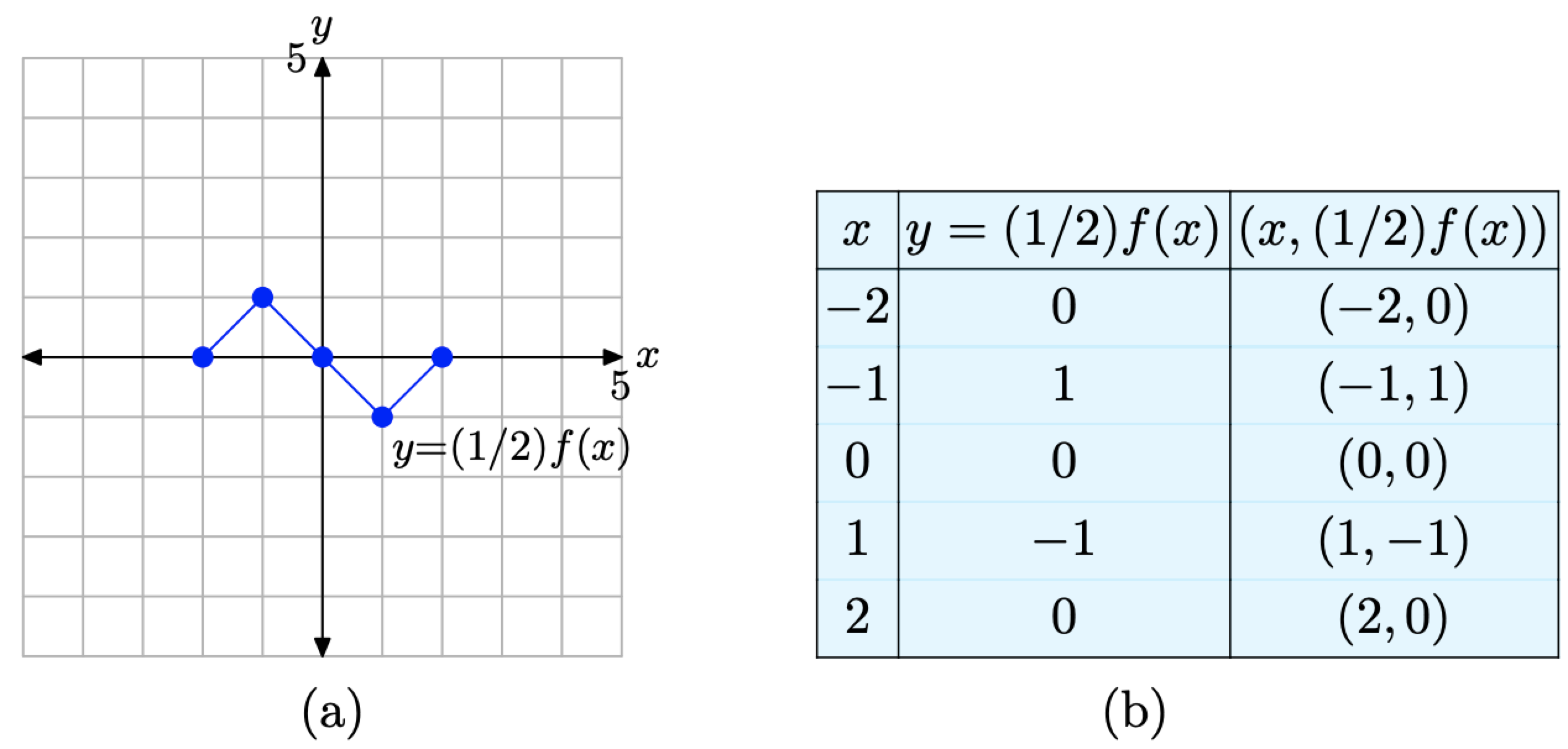
Figure \(\PageIndex{5}\). The points in the table are points on the graph of y = (1/2)f(x).

Note the result. The graph of f has been compressed vertically (toward the x-axis), both positively and negatively, by a factor of 2.

Let’s summarize our findings.

A Visual Summary — Vertical Scaling.

Consider the images in Figure \(\PageIndex{6}\).

• In Figure \(\PageIndex{6}\)(a), we see pictured the graph of the original function y = f(x).
• In Figure \(\PageIndex{6}\)(b), note that each key point on the graph of y = 2f(x) has a y-value that is precisely double the y-value of the corresponding point on the graph of y = f(x) in Figure \(\PageIndex{6}\)(a).
• In Figure \(\PageIndex{6}\)(c), note that each key point on the graph of y = (1/2)f(x) has a y-value that is precisely half the y-value of the corresponding point on the graph of y = f(x) in Figure \(\PageIndex{6}\)(a).
• Note that the x-value of each transformed point remains the same.

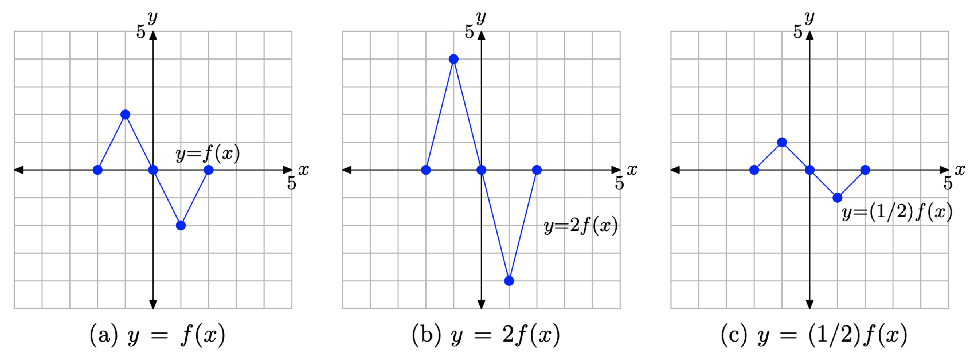
Figure \(\PageIndex{6}\). The graph of y = 2f(x) stretches vertically (away from the x-axis) by a factor of 2. The graph of y = (1/2)f(x) compresses vertically (toward the x-axis) by a factor of 2.

The visual summary in Figure \(\PageIndex{6}\) makes sketching the graphs of y = 2f(x) and y = (1/2)f(x) an easy task.

• Given the graph of y = f(x), to sketch the graph of y = 2f(x), simply take each point on the graph of y = f(x) and double its y-value, keeping the same x-value.
• Given the graph of y = f(x), to sketch the graph of y = (1/2)f(x), simply take each point on the graph of y = f(x) and halve its y-value, keeping the same x-value.

Follow the same procedures for other scaling factors. For example, in the case of y = 3f(x), take each point on the graph of y = f(x) and multiply its y-value by 3, keeping the same x-value. On the other hand, to draw the graph of y = (1/3)f(x), take each point on the graph of f and multiply its y-value by 1/3, keeping the same y-value.

In general, we can state the following.

summary

Suppose we are given the graph of y = f(x).

• If a > 1, then the graph of y = af(x) is stretched vertically (away from the x-axis), both positively and negatively, by a factor of a.
• If 0 < a < 1, then the graph of y = af(x) is compressed vertically (toward the x-axis), both positively and negatively, by a factor of 1/a.

The second item in Summary warrants a word of explanation. Compare the general form y = af(x) with the function of Example \(\PageIndex{3}\), y = (1/2)f(x). In this case, a = 1/2, so \[\frac{1}{a}=\frac{1}{1 / 2}=1 \times 2=2 \nonumber \]

The second item says that when 0 < a < 1, the graph of y = af(x) is compressed vertically by a factor of 1/a. Indeed, this is exactly what happens in the case of y = (1/2)f(x), which is compressed by a factor of 1/(1/2), or 2.

Vertical Reflections

For convenience, we begin by repeating the original graph of y = f(x) and its accompanying data.

We are now going to reflect the graph in the vertical direction (across the x-axis).

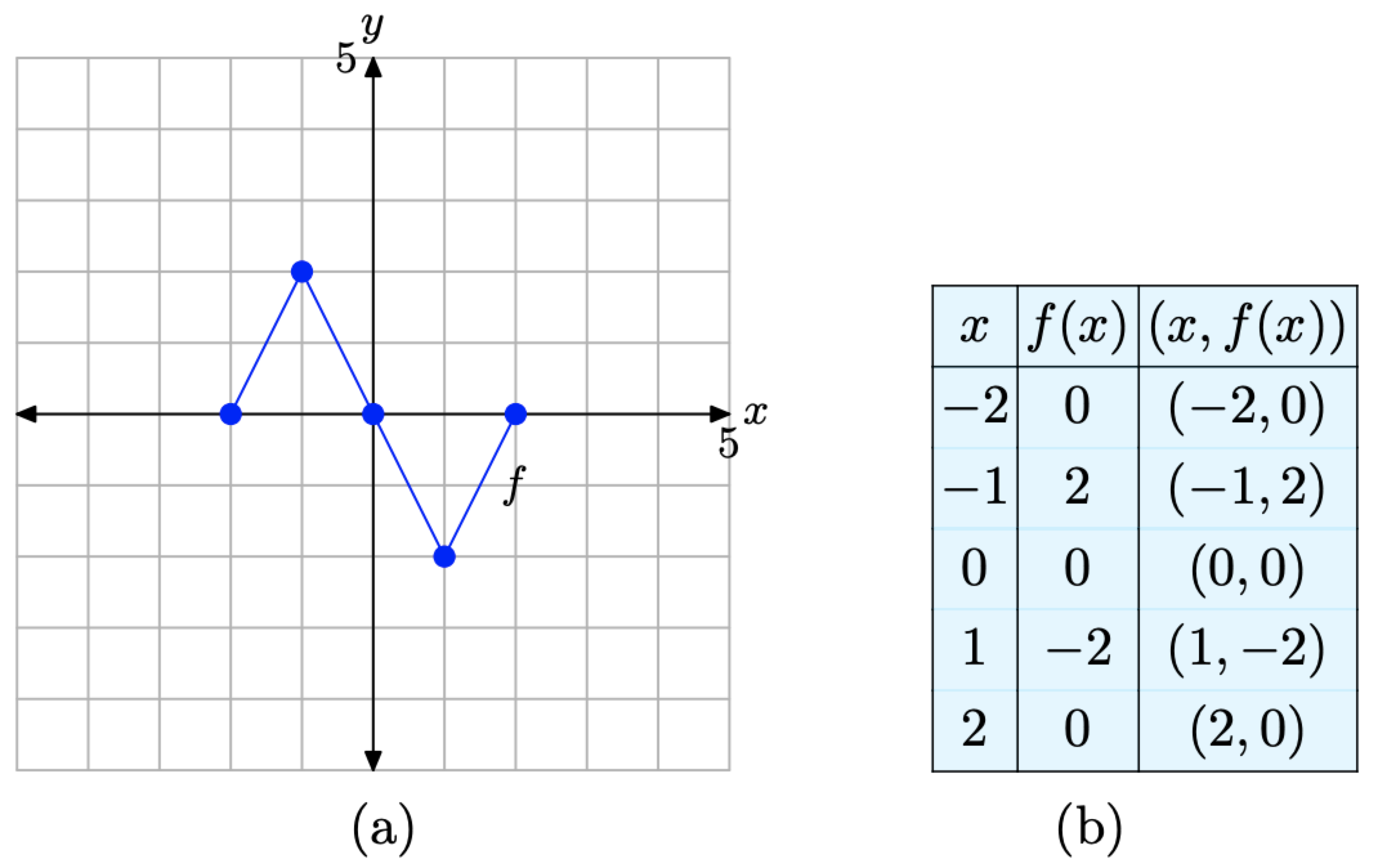
Figure \(\PageIndex{7}\). The original graph of f and a table of key points on the graph of f.

Example \(\PageIndex{4}\)

If y = f(x) has the graph shown in Figure \(\PageIndex{7}\)(a), sketch the graph of y = −f(x).

Solution

To set up a table of points in preparation for the plot of y = −f(x), we’ll use exactly the same values of x that you see in the table in Figure \(\PageIndex{7}\)(b), namely x = −2, −1, 0, 1, and 2. To evaluate y = −f(x) at the first value of x, namely x = −2, we make the following calculation,

\[y=-f(-2)=-(0)=0 \nonumber \]

where we’ve used the fact that f(−2) = 0 from the table in Figure \(\PageIndex{7}\)(b). In similar fashion, we evaluate y = −f(x) at each of the remaining values of x, namely x = −1, 0, 1, and 2.

\[\begin{aligned} y &=-f(-1)=-(2)=-2 \\ y &=-f(0)=-(0)=0 \\ y &=-f(1)=-(-2)=2 \\ y &=-f(2)=-(0)=0 \end{aligned} \nonumber \]

We assemble these points in the table in Figure \(\PageIndex{8}\)(b) and plot them in Figure \(\PageIndex{8}\)(a).

Note that the graph of y = −f(x) in Figure \(\PageIndex{8}\)(a) is a reflection of the graph of y = f(x) in Figure \(\PageIndex{7}\)(a) across the x-axis.

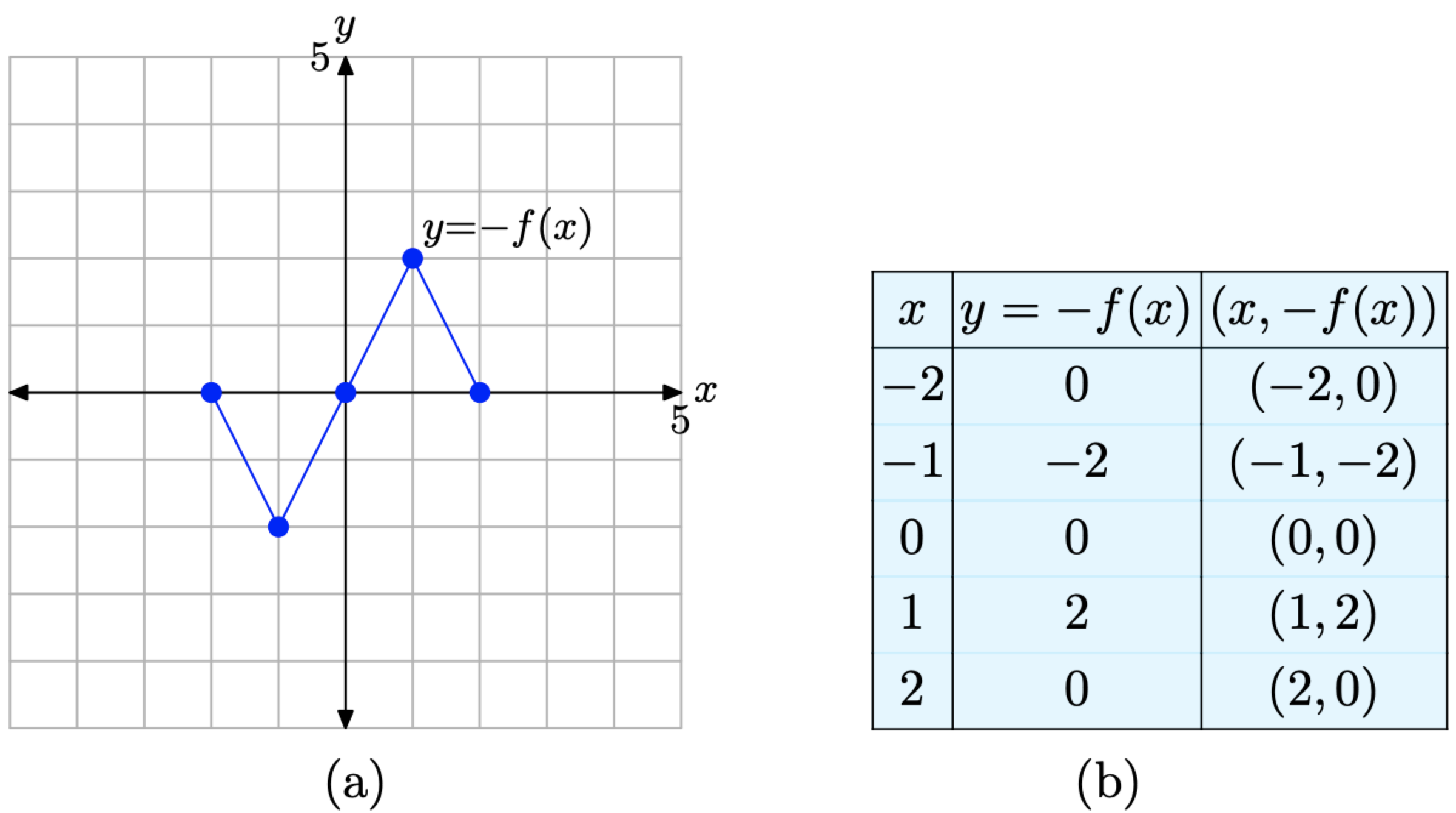
Figure \(\PageIndex{8}\). The graph of y = −f(x) and a table of key points on the graph.

Let’s summarize what we’ve learned about vertical reflections.

A Visual Summary — Vertical Reflections

Consider the images in Figure \(\PageIndex{9}\).

• In Figure \(\PageIndex{9}\)(a), we see pictured the original graph of y = f(x).
• In Figure \(\PageIndex{9}\)(b), the graph of y = −f(x) is a reflection of the graph of y = f(x) across the x-axis.

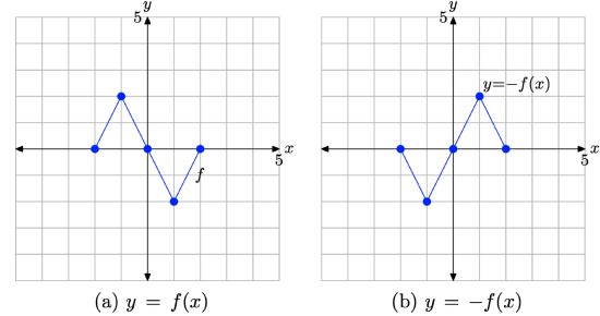
Figure \(\PageIndex{9}\). The graph of y = −f(x) is a reflection of the graph of y = f(x) across the x-axis.

Thus, given the graph of y = f(x), it is a simple task to draw the graph of y = −f(x).

• To draw the graph of y = −f(x), take each point on the graph of y = f(x) and reflect it across the x-axis, keeping the x-value the same, but negating the y-value.

Vertical Translations

Translations are perhaps the easiest transformation of all. A translation is a “shift” or a “slide.” Pretend, for a moment, that you’ve placed a transparent sheet of thin plastic over a sheet of graph paper. You’ve drawn a Cartesian coordinate system on your graph paper, but you’ve plotted your graph on the transparent sheet of plastic. Now, “shift” or “slide” the transparency over your graph paper in a constant direction without rotating the transparency. This is what we mean by a “translation.” In this section, we will focus strictly on vertical translations.

For convenience, we begin by repeating the original graph of y = f(x) and its accompanying data in Figure \(\PageIndex{10}\)(a) and( b), respectively. We will now translate this graph in the vertical direction.

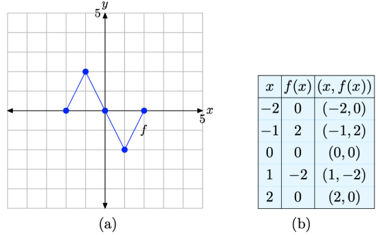
Figure \(\PageIndex{10}\). The original graph of f and a table of key points on the graph of f.

Example \(\PageIndex{5}\)

If y = f(x) has the graph shown in Figure \(\PageIndex{10}\)(a), sketch the graph of y = f(x) + 1.

Solution

We will evaluate y = f(x)+1 at the same values shown in the table in Figure \(\PageIndex{10}\)(b), namely x = −2, −1, 0, 1, and 2. To evaluate y = f(x)+1 at the first value of x, namely x = −2, we make the following calculation \[y=f(-2)+1=0+1=1 \nonumber \]

where we’ve used that fact that f(−2) = 0 from the table in Figure \(\PageIndex{10}\)(b). In similar fashion, we can evaluate y = f(x) + 1 at each of the remaining values of x, namely x = −1, 0, 1, and 2.

\[\begin{array}{l}{y=f(-1)+1=2+1=3} \\ {y=f(0)+1=0+1=1} \\ {y=f(1)+1=-2+1=-1} \\ {y=f(2)+1=0+1=1}\end{array} \nonumber \]

We assemble these points in the table in Figure \(\PageIndex{11}\)(b) and plot them in Figure \(\PageIndex{11}\)(a).

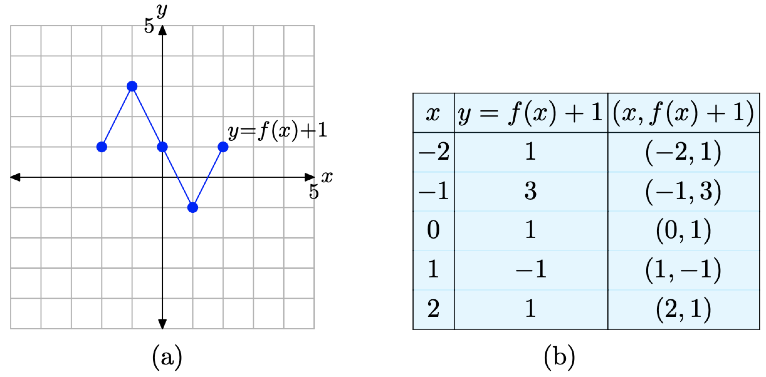
Figure \(\PageIndex{11}\). The graph of y = f(x) + 1 and a table of key points on the graph.

When you compare the entries in the table in Figure \(\PageIndex{11}\).(b) with the original values in the table in Figure \(\PageIndex{10}\).(b), you’ll note that the x-values in each table are identical, but the y-values in the table in Figure \(\PageIndex{11}\).(b) are all increased by 1. This makes sense, because these are the y-values of the points associated with the function y = f(x) + 1. Of course, all the y-values should be 1 larger than the y-values associated with the original equation y = f(x).

Note the result. The graph of y = f(x) + 1 in Figure \(\PageIndex{11}\)(a), when compared with the graph of y = f(x) in Figure \(\PageIndex{10}\)(a), is shifted 1 unit upwards.

Let’s look at another example.

Example \(\PageIndex{6}\)

If y = f(x) has the graph shown in Figure \(\PageIndex{10}\)(a), sketch the graph of y = f(x) − 2.

Solution

Evaluate the function y = f(x) − 2 at each value of x in the table in Figure \(\PageIndex{10}\)(b). At x = −2, \[y=f(-2)-2=0-2=-2 \nonumber \]

In similar fashion, evaluate y = f(x) − 2 at each remaining x-value in the table in Figure \(\PageIndex{10}\)(b).

\[\begin{aligned} y &=f(-1)-2=2-2=0 \\ y &=f(0)-2=0-2=-2 \\ y &=f(1)-2=-2-2=-4 \\ y &=f(2)-2=0-2=-2 \end{aligned} \nonumber \]

We assemble these points in the table in Figure \(\PageIndex{12}\)(b) and plot them in Figure \(\PageIndex{12}\)(a).

When you compare the entries in the table in Figure \(\PageIndex{12}\)(b) with the original values in the table in Figure \(\PageIndex{10}\)(b), you’ll note that the x-values in each table are identical, but the y-values in the table in Figure \(\PageIndex{12}\)(b) are all decremented by 2. This makes

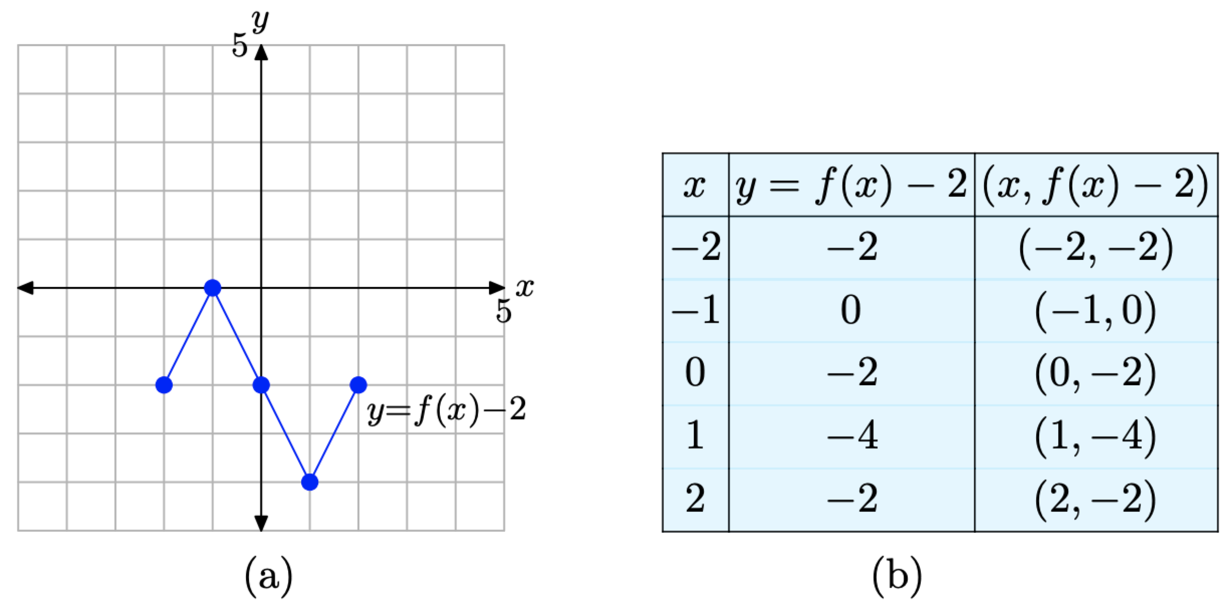
Figure \(\PageIndex{12}\). The graph of y = f(x) − 2 and a table of key points on the graph.

sense, because these are the y-values of the points associated with the function y = f(x) − 2. Of course, all the y-values should be 2 less than the y-values associated with the original equation y = f(x).

Note the result. The graph of y = f(x) − 2 in Figure \(\PageIndex{12}\)(a), when compared with the graph of y = f(x) in Figure \(\PageIndex{10}\)(a), is shifted downward 2 units.

Let’s summarize what we’ve learned about vertical translations.

A Visual Summary — Vertical Translations (Shifts)

Consider the images in Figure \(\PageIndex{13}\).

• In Figure \(\PageIndex{13}\)(a), we see pictured the graph of the original function y = f(x).
• In Figure \(\PageIndex{13}\)(b), note that each key point on the graph of y = f(x) + 1 has a y-value that is precisely 1 unit larger than the y-value of the corresponding point on the graph of y = f(x) in in Figure \(\PageIndex{13}\)(a).
• In Figure \(\PageIndex{13}\)(c), note that each key point on the graph of y = f(x) − 2 has a y-value that is precisely 2 units smaller than the y-value of the corresponding point on the graph of y = f(x) in in Figure \(\PageIndex{13}\)(a).
• Note that the x-value of each transformed point remains the same.

The visual summary in Figure \(\PageIndex{13}\) makes sketching the graphs of y = f(x) + 1 and y = f(x) − 2 an easy task.

• Given the graph of y = f(x), to sketch the graph of y = f(x) + 1, simply take each point on the graph of y = f(x) and move it upwards 1 unit, keeping the same x-value.
• Given the graph of y = f(x), to sketch the graph of y = f(x) − 2, simply take each point on the graph of y = f(x) and move it downwards 2 units, keeping the same x-value.

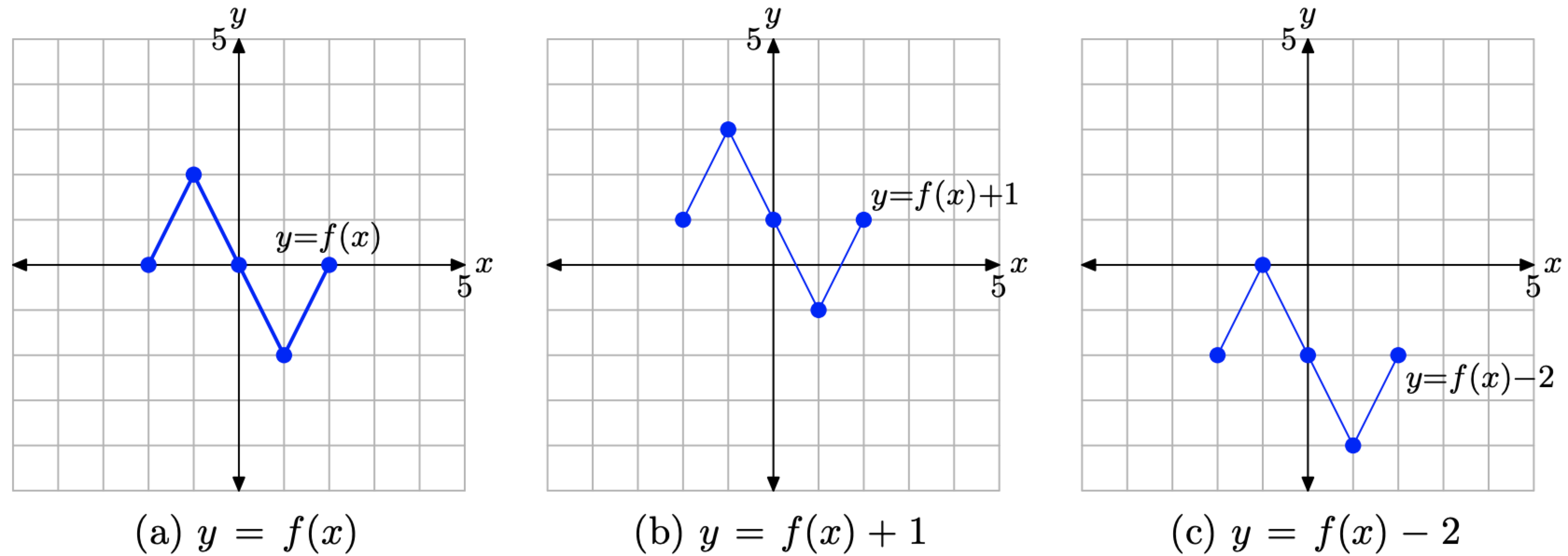
Figure \(\PageIndex{13}\). The graph of y = f(x) + 1 is formed by shifting (vertically) the graph of y = f(x) upward 1 unit. The graph of y = f(x) − 2 is formed by shifting (vertically) the graph of y = f(x) downward 2 units.

In general, we can state the following.

summary

Suppose that we are given the graph of y = f(x) and suppose that c is any positive real number.

• The graph of y = f(x)+c is shifted c units upward from the graph of y = f(x).
• The graph of y = f(x) − c is shifted c units downward from the graph of y = f(x).

Composing Transformations

Sometimes we will want to perform one transformation, then take the result of the first transformation and apply a second transformation. Let’s look at an example.

Example \(\PageIndex{7}\)

Consider the graph of y = f(x) presented in Figure \(\PageIndex{14}\).

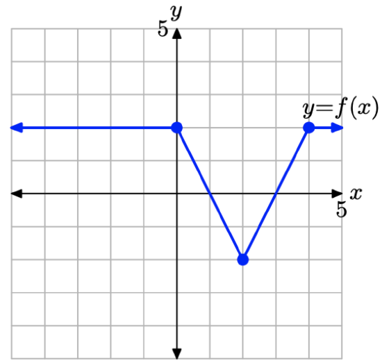
Figure \(\PageIndex{14}\) The graph of y = f(x) that will be transformed in Example \(\PageIndex{7}\).

Use the concepts discussed in the Visual Summaries to sketch the graph of y = −2f(x) without creating and referring to a table of points.

Solution

Note that the equation y = −2f(x) can be formed by a sequence of two transformations.

1. First, scale the original function y = f(x) to obtain the equation y = 2f(x).
2. Second, negate the resulting function y = 2f(x) to obtain the equation y = −2f(x).

Thus, the graph of y = −2f(x) can be formed as follows:

1. Start with the graph of y = f(x) and double the y-value of each point on the graph of y = f(x), keeping the same x-value. The result is the graph of y = 2f(x) shown in Figure \(\PageIndex{15}\)(b).
2. Next, negate the y-value of each point on the graph of y = 2f(x), keeping the same x-value. The result is the graph of y = −2f(x) in Figure \(\PageIndex{15}\)(c).

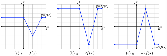
Figure \(\PageIndex{15}\). Transforming the graph of y = f(x) with a sequence of two transformations.

It is interesting to note that you will get the same result if you negate first, then scale the result. We will leave it to our readers to check that this is true.

Let’s look at one final example.

Example \(\PageIndex{8}\)

Consider the graph of y = f(x) presented in Figure \(\PageIndex{16}\).

Use the concepts discussed in the Visual Summaries to sketch the graph of y = −f(x)+2 without creating and referring to a table of points.

Solution

Note that the equation y = −f(x) + 2 can be formed by a sequence of two transformations.

1. First, negate the original function y = f(x) to obtain the equation y = −f(x).
2. Second, add 2 to the resulting function y = −f(x) to obtain the equation y = −f(x) + 2.

Thus, the graph of y = −f(x) + 2 can be formed as follows.

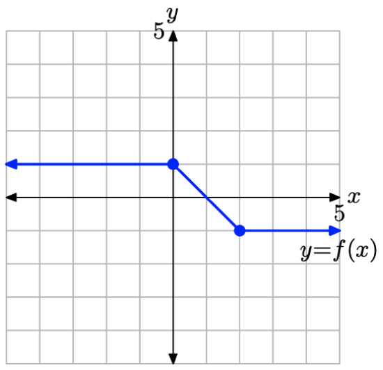
Figure \(\PageIndex{16}\). The graph of y = f(x) that will be transformed in Example \(\PageIndex{8}\).

1. First, start with the graph of y = f(x) in Figure \(\PageIndex{17}\)(a) and negate the y-value of each point to produce the graph of y = −f(x) Figure \(\PageIndex{17}\)(b).

2. Next, add 2 to the y-value of each point on the graph of y = −f(x) in Figure \(\PageIndex{17}\)(b) to produce the graph of y = −f(x) + 2 in Figure \(\PageIndex{17}\)(c).

Figure \(\PageIndex{17}\). Transforming the graph of y = f(x), first reflecting across the x-axis, then shifting 2 units upward to obtain the graph of y = −f(x) + 2.

In Example \(\PageIndex{7}\), where we started with the graph of y = f(x) and then graphed y = 2f(x), the order of the transformations did not matter. Scale by 2, then negate, or negate and scale by 2, you get the same result (readers should verify this claim). However, in this example, the order in which the transformations are applied does matter. To see this, let’s do the following:

1. Add 2 to shift the graph of y = f(x) in Figure \(\PageIndex{18}\)(a) two units upward to obtain the graph of y = f(x) + 2 in Figure \(\PageIndex{18}\)(b).
2. Negate the y-value of each point on the graph of y = f(x) + 2 in Figure \(\PageIndex{18}\)(b) to obtain the graph of y = −(f(x) + 2) in Figure \(\PageIndex{18}\)(c). Note that we must negate the entire y-value. Hence the parentheses.

Unfortunately, the graph of y = −(f(x)+ 2) in Figure \(\PageIndex{18}\)(c) is not the same as the graph of y = −f(x) + 2 in Figure \(\PageIndex{17}\)(c). But of course, this makes complete sense, as the equations (in the case of Figure \(\PageIndex{18}\)(c))

\[y=-(f(x)+2)=-f(x)-2 \nonumber \]

and (in the case of Figure \(\PageIndex{17}\)(c))

\[y=-f(x)+2 \nonumber \]

are also not the same.

Figure \(\PageIndex{18}\). Transforming the graph of y = f(x), shifting 2 units upward to obtain the graph of y = f(x) + 2, then reflecting across the x-axis to obtain the graph of y = −(f(x) + 2).

Therefore, care must be taken when applying more than one transformation. Here is a good rule of thumb to live by.

Do Vertical Scalings and Reflections First, then Vertical Translations. When performing a sequence of vertical transformations, it is usually easier (less confusing) to apply vertical scalings and reflections before vertical translations.

However, as long as you perform the transformations correctly, you should obtain the correct result. In Example \(\PageIndex{8}\), if you want to sketch the graph of y = −f(x)+2 by doing the translation first, the correct way to proceed is as follows (though somewhat counterintuitive):

1. First, shift the graph of y = f(x) downward 2 units to obtain the graph of y = f(x) − 2.
2. Second, reflect the graph of y = f(x) − 2 across the x-axis to obtain the graph of y = −(f(x) − 2). Again, note the use of parentheses as we negate the entire y-value.

Finally, note that \[y=-(f(x)-2)=-f(x)+2 \nonumber \]

We will leave it to our readers to show that this sequence produces the correct result, a graph identical to the correct answer shown in Figure \(\PageIndex{17}\)(c).

Summary

In this section we’ve seen how a handful of transformations greatly enhance our graphing capability. We end this section by listing the transformations presented in this section and their effects on the graph of a function.

Vertical Transformations.

Vertical Transformations. Suppose we are given the graph of y = f(x).

• If \(a > 1\), then the graph of y = af(x) is stretched vertically (away from the x-axis), both positively and negatively, by a factor of a.
• If \(0 < a < 1\), then the graph of y = af(x) is compressed vertically (toward the x-axis), both positively and negatively, by a factor of 1/a.
• The graph of y = −f(x) is a reflection of the graph of y = f(x) across the x-axis.
• If \(c > 0\), then the graph of y = f(x) + c is shifted c units upward from the graph of y = f(x).
• If \(c > 0\), then the graph of y = f(x) − c is shifted c units downward from the graph of y = f(x).