
7.1: Introducing Rational Functions
- Page ID
- 19720

\( \newcommand{\vecs}[1]{\overset { \scriptstyle \rightharpoonup} {\mathbf{#1}} } \)
\( \newcommand{\vecd}[1]{\overset{-\!-\!\rightharpoonup}{\vphantom{a}\smash {#1}}} \)
\( \newcommand{\dsum}{\displaystyle\sum\limits} \)
\( \newcommand{\dint}{\displaystyle\int\limits} \)
\( \newcommand{\dlim}{\displaystyle\lim\limits} \)
\( \newcommand{\id}{\mathrm{id}}\) \( \newcommand{\Span}{\mathrm{span}}\)
( \newcommand{\kernel}{\mathrm{null}\,}\) \( \newcommand{\range}{\mathrm{range}\,}\)
\( \newcommand{\RealPart}{\mathrm{Re}}\) \( \newcommand{\ImaginaryPart}{\mathrm{Im}}\)
\( \newcommand{\Argument}{\mathrm{Arg}}\) \( \newcommand{\norm}[1]{\| #1 \|}\)
\( \newcommand{\inner}[2]{\langle #1, #2 \rangle}\)
\( \newcommand{\Span}{\mathrm{span}}\)
\( \newcommand{\id}{\mathrm{id}}\)
\( \newcommand{\Span}{\mathrm{span}}\)
\( \newcommand{\kernel}{\mathrm{null}\,}\)
\( \newcommand{\range}{\mathrm{range}\,}\)
\( \newcommand{\RealPart}{\mathrm{Re}}\)
\( \newcommand{\ImaginaryPart}{\mathrm{Im}}\)
\( \newcommand{\Argument}{\mathrm{Arg}}\)
\( \newcommand{\norm}[1]{\| #1 \|}\)
\( \newcommand{\inner}[2]{\langle #1, #2 \rangle}\)
\( \newcommand{\Span}{\mathrm{span}}\) \( \newcommand{\AA}{\unicode[.8,0]{x212B}}\)
\( \newcommand{\vectorA}[1]{\vec{#1}} % arrow\)
\( \newcommand{\vectorAt}[1]{\vec{\text{#1}}} % arrow\)
\( \newcommand{\vectorB}[1]{\overset { \scriptstyle \rightharpoonup} {\mathbf{#1}} } \)
\( \newcommand{\vectorC}[1]{\textbf{#1}} \)
\( \newcommand{\vectorD}[1]{\overrightarrow{#1}} \)
\( \newcommand{\vectorDt}[1]{\overrightarrow{\text{#1}}} \)
\( \newcommand{\vectE}[1]{\overset{-\!-\!\rightharpoonup}{\vphantom{a}\smash{\mathbf {#1}}}} \)
\( \newcommand{\vecs}[1]{\overset { \scriptstyle \rightharpoonup} {\mathbf{#1}} } \)
\(\newcommand{\longvect}{\overrightarrow}\)
\( \newcommand{\vecd}[1]{\overset{-\!-\!\rightharpoonup}{\vphantom{a}\smash {#1}}} \)
\(\newcommand{\avec}{\mathbf a}\) \(\newcommand{\bvec}{\mathbf b}\) \(\newcommand{\cvec}{\mathbf c}\) \(\newcommand{\dvec}{\mathbf d}\) \(\newcommand{\dtil}{\widetilde{\mathbf d}}\) \(\newcommand{\evec}{\mathbf e}\) \(\newcommand{\fvec}{\mathbf f}\) \(\newcommand{\nvec}{\mathbf n}\) \(\newcommand{\pvec}{\mathbf p}\) \(\newcommand{\qvec}{\mathbf q}\) \(\newcommand{\svec}{\mathbf s}\) \(\newcommand{\tvec}{\mathbf t}\) \(\newcommand{\uvec}{\mathbf u}\) \(\newcommand{\vvec}{\mathbf v}\) \(\newcommand{\wvec}{\mathbf w}\) \(\newcommand{\xvec}{\mathbf x}\) \(\newcommand{\yvec}{\mathbf y}\) \(\newcommand{\zvec}{\mathbf z}\) \(\newcommand{\rvec}{\mathbf r}\) \(\newcommand{\mvec}{\mathbf m}\) \(\newcommand{\zerovec}{\mathbf 0}\) \(\newcommand{\onevec}{\mathbf 1}\) \(\newcommand{\real}{\mathbb R}\) \(\newcommand{\twovec}[2]{\left[\begin{array}{r}#1 \\ #2 \end{array}\right]}\) \(\newcommand{\ctwovec}[2]{\left[\begin{array}{c}#1 \\ #2 \end{array}\right]}\) \(\newcommand{\threevec}[3]{\left[\begin{array}{r}#1 \\ #2 \\ #3 \end{array}\right]}\) \(\newcommand{\cthreevec}[3]{\left[\begin{array}{c}#1 \\ #2 \\ #3 \end{array}\right]}\) \(\newcommand{\fourvec}[4]{\left[\begin{array}{r}#1 \\ #2 \\ #3 \\ #4 \end{array}\right]}\) \(\newcommand{\cfourvec}[4]{\left[\begin{array}{c}#1 \\ #2 \\ #3 \\ #4 \end{array}\right]}\) \(\newcommand{\fivevec}[5]{\left[\begin{array}{r}#1 \\ #2 \\ #3 \\ #4 \\ #5 \\ \end{array}\right]}\) \(\newcommand{\cfivevec}[5]{\left[\begin{array}{c}#1 \\ #2 \\ #3 \\ #4 \\ #5 \\ \end{array}\right]}\) \(\newcommand{\mattwo}[4]{\left[\begin{array}{rr}#1 \amp #2 \\ #3 \amp #4 \\ \end{array}\right]}\) \(\newcommand{\laspan}[1]{\text{Span}\{#1\}}\) \(\newcommand{\bcal}{\cal B}\) \(\newcommand{\ccal}{\cal C}\) \(\newcommand{\scal}{\cal S}\) \(\newcommand{\wcal}{\cal W}\) \(\newcommand{\ecal}{\cal E}\) \(\newcommand{\coords}[2]{\left\{#1\right\}_{#2}}\) \(\newcommand{\gray}[1]{\color{gray}{#1}}\) \(\newcommand{\lgray}[1]{\color{lightgray}{#1}}\) \(\newcommand{\rank}{\operatorname{rank}}\) \(\newcommand{\row}{\text{Row}}\) \(\newcommand{\col}{\text{Col}}\) \(\renewcommand{\row}{\text{Row}}\) \(\newcommand{\nul}{\text{Nul}}\) \(\newcommand{\var}{\text{Var}}\) \(\newcommand{\corr}{\text{corr}}\) \(\newcommand{\len}[1]{\left|#1\right|}\) \(\newcommand{\bbar}{\overline{\bvec}}\) \(\newcommand{\bhat}{\widehat{\bvec}}\) \(\newcommand{\bperp}{\bvec^\perp}\) \(\newcommand{\xhat}{\widehat{\xvec}}\) \(\newcommand{\vhat}{\widehat{\vvec}}\) \(\newcommand{\uhat}{\widehat{\uvec}}\) \(\newcommand{\what}{\widehat{\wvec}}\) \(\newcommand{\Sighat}{\widehat{\Sigma}}\) \(\newcommand{\lt}{<}\) \(\newcommand{\gt}{>}\) \(\newcommand{\amp}{&}\) \(\definecolor{fillinmathshade}{gray}{0.9}\)In the previous chapter, we studied polynomials, functions having equation form
\[p(x)=a_{0}+a_{1} x+a_{2} x^{2}+\cdots+a_{n} x^{n} \nonumber \]
Even though this polynomial is presented in ascending powers of \(x\), the leading term of the polynomial is still \(a_{n} x^{n}\), the term with the highest power of \(x\). The degree of the polynomial is the highest power of (x\) present, so in this case, the degree of the polynomial is \(n\).
In this section, our study will lead us to the rational functions. Note the root word “ratio” in the term “rational.” Does it remind you of the word “fraction”? It should, as rational functions are functions in a very specific fractional form.
A rational function is a function that can be written as a quotient of two polynomial functions. In symbols, the function
\[f(x)=\frac{a_{0}+a_{1} x+a_{2} x^{2}+\cdots+a_{n} x^{n}}{b_{0}+b_{1} x+b_{2} x^{2}+\cdots+b_{m} x^{m}} \nonumber \]
is called a rational function.
For example,
\[f(x)=\frac{1+x}{x+2}, \quad g(x)=\frac{x^{2}-2 x-3}{x+4}, \quad \text { and } \quad h(x)=\frac{3-2 x-x^{2}}{x^{3}+2 x^{2}-3 x-5} \label{4} \]
are rational functions, while
\[f(x)=\frac{1+\sqrt{x}}{x^{2}+1}, \quad g(x)=\frac{x^{2}+2 x-3}{1+x^{1 / 2}-3 x^{2}}, \quad \text { and } \quad h(x)=\sqrt{\frac{x^{2}-2 x-3}{x^{2}+4 x-12}} \label{5} \]
are not rational functions.
Each of the functions in Equation \ref{4} are rational functions, because in each case, the numerator and denominator of the given expression is a valid polynomial.
However, in Equation \ref{5}, the numerator of \(f(x)\) is not a polynomial (polynomials do not allow the square root of the independent variable). Therefore, \(f\) is not a rational function. Similarly, the denominator of \(g(x)\) in Equation \ref{5} is not a polynomial. Fractions are not allowed as exponents in polynomials. Thus, \(g\) is not a rational function. Finally, in the case of function \(h\) in Equation \ref{5}, although the radicand (the expression inside the radical) is a rational function, the square root prevents h from being a rational function.
An important skill to develop is the ability to draw the graph of a rational function. Let’s begin by drawing the graph of one of the simplest (but most fundamental) rational functions.
The Graph of y = 1/x
In all new situations, when we are presented with an equation whose graph we’ve not considered or do not recognize, we begin the process of drawing the graph by creating a table of points that satisfy the equation. It’s important to remember that the graph of an equation is the set of all points that satisfy the equation. We note that zero is not in the domain of \(y = 1/x\) (division by zero makes no sense and is not defined), and create a table of points satisfying the equation shown in Figure \(\PageIndex{1}\).
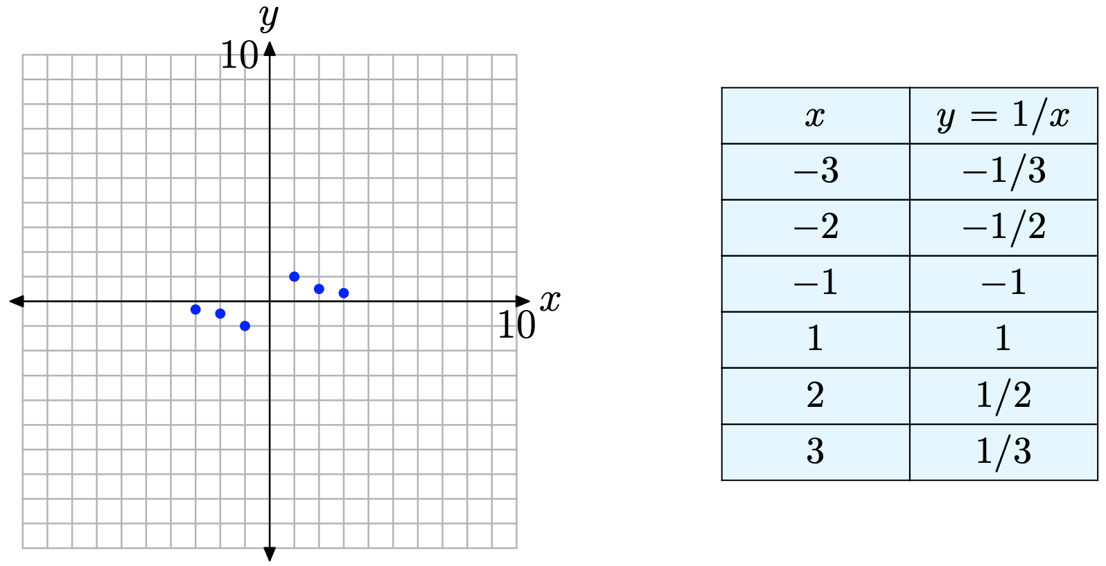
At this point (Figure \(\PageIndex{1}\)), it’s pretty clear what the graph is doing between \(x = −3\) and \(x = −1\). Likewise, it’s clear what is happening between x = 1 and x = 3. However, there are some open areas of concern.
- What happens to the graph as x increases without bound? That is, what happens to the graph as x moves toward \(\infty\)?
- What happens to the graph as x decreases without bound? That is, what happens to the graph as x moves toward \(-\infty\)?
- What happens to the graph as x approaches zero from the right?
- What happens to the graph as x approaches zero from the left?
Let’s answer each of these questions in turn. We’ll begin by discussing the “endbehavior” of the rational function defined by y = 1/x. First, the right end. What happens as x increases without bound? That is, what happens as x increases toward ∞? In Table \(\PageIndex{1a}\), we computed y = 1/x for x equaling 100, 1000, and 10000. Note how the y-values in Table \(\PageIndex{1a}\) are all positive and approach zero.
Students in calculus use the following notation for this idea.
\[\lim _{x \rightarrow \infty} y=\lim _{x \rightarrow \infty} \frac{1}{x}=0 \nonumber \]
They say “the limit of y as x approaches infinity is zero.” That is, as x approaches infinity, y approaches zero.
| x | y = 1/x |
|---|---|
| 100 | 0.01 |
| 1000 | 0.001 |
| 10000 | 0.0001 |
A completely similar event happens at the left end. As x decreases without bound, that is, as x decreases toward \(-\infty\), note that the y-values in Table \(\PageIndex{1}\)(b) are all negative and approach zero. Calculus students have a similar notation for this idea.
\[\lim _{x \rightarrow-\infty} y=\lim _{x \rightarrow-\infty} \frac{1}{x}=0 \nonumber \]
They say “the limit of y as x approaches negative infinity is zero.” That is, as x approaches negative infinity, y approaches zero.
| x | y=1/x |
|---|---|
| -100 | -0.01 |
| -1000 | -0.001 |
| -10000 | -0.0001 |
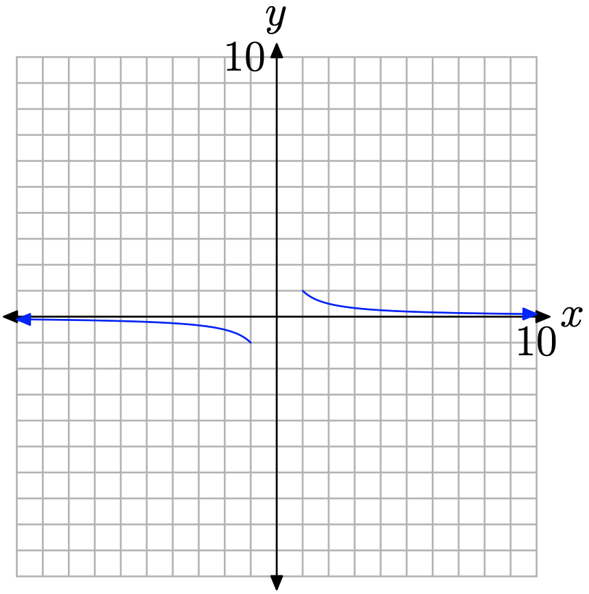
These numbers in Tables \(\PageIndex{1a}\) and \(\PageIndex{1b}\), and the ideas described above, predict the correct end-behavior of the graph of \(y = 1/x\). At each end of the x-axis, the y-values must approach zero. This means that the graph of \(y = 1/x\) must approach the x-axis for x-values at the far right- and left-ends of the graph. In this case, we say that the x-axis acts as a horizontal asymptote for the graph of \(y = 1/x\). As \(x\) approaches either positive or negative infinity, the graph of \(y = 1/x\) approaches the x-axis. This behavior is shown in Figure \(\PageIndex{2}\).
Our last investigation will be on the interval from \(x = −1\) to \(x = 1\). Readers are again reminded that the function y = 1/x is undefined at x = 0. Consequently, we will break this region in half, first investigating what happens on the region between x = 0 and x = 1. We evaluate y = 1/x at x = 1/2, x = 1/4, and x = 1/8, as shown in the table in Figure \(\PageIndex{3}\), then plot the resulting points.
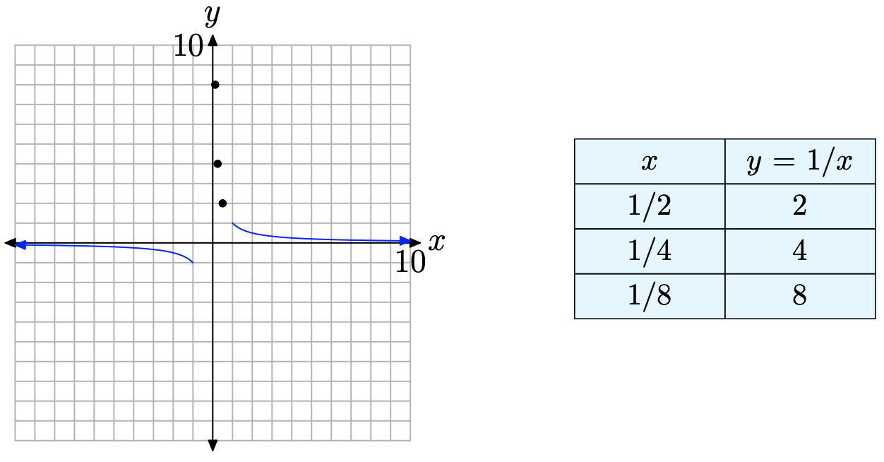
Note that the x-values in the table in Figure \(\PageIndex{3}\) approach zero from the right, then note that the corresponding y-values are getting larger and larger. We could continue in this vein, adding points. For example, if \(x = 1/16\), then \(y = 16\). If \(x = 1/32\), then \(y = 32\). If \(x = 1/64\), then \(y = 64\). Each time we halve our value of x, the resulting value of x is closer to zero, and the corresponding y-value doubles in size. Calculus students describe this behavior with the notation
\[\lim _{x \rightarrow 0^{+}} y=\lim _{x \rightarrow 0^{+}} \frac{1}{x}=\infty \nonumber \]
That is, as “x approaches zero from the right, the value of y grows to infinity.” This is evident in the graph in Figure \(\PageIndex{3}\), where we see the plotted points move closer to the vertical axis while at the same time moving upward without bound. A similar thing happens on the other side of the vertical axis, as shown in Figure \(\PageIndex{4}\).
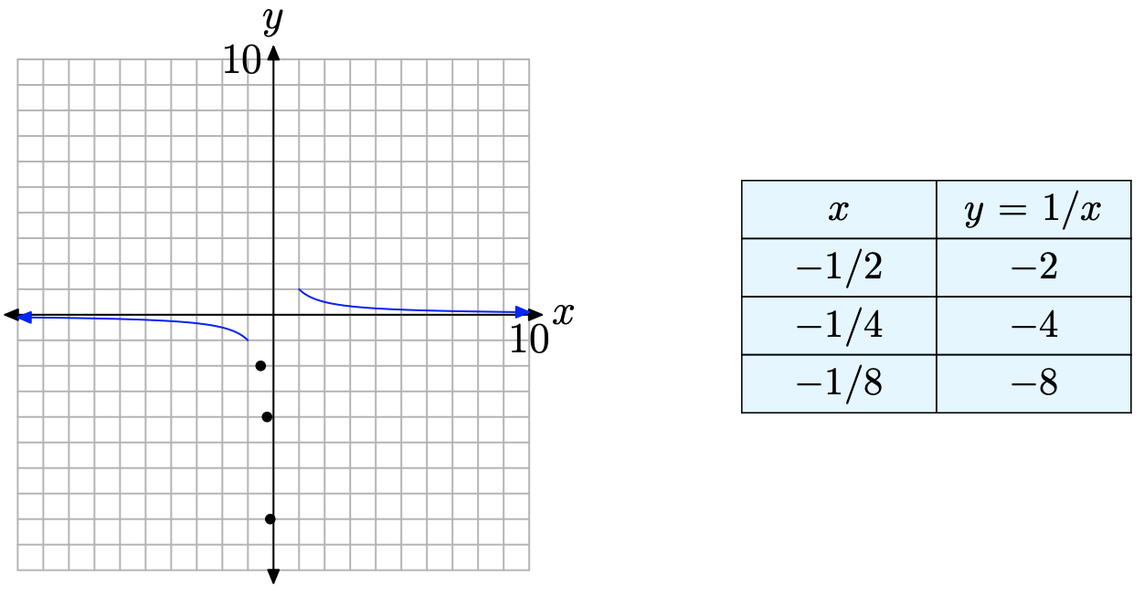
Again, calculus students would write \[\lim _{x \rightarrow 0^{-}} y=\lim _{x \rightarrow 0^{-}} \frac{1}{x}=-\infty \nonumber \]
That is, “as x approaches zero from the left, the values of y decrease to negative infinity.” In Figure \(\PageIndex{4}\), it is clear that as points move closer to the vertical axis (as x approaches zero) from the left, the graph decreases without bound. The evidence gathered to this point indicates that th
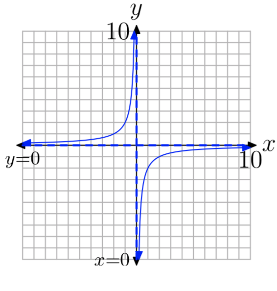
The evidence gathered to this point indicates that the vertical axis is acting as a vertical asymptote. As x approaches zero from either side, the graph approaches the vertical axis, either rising to infinity, or falling to negative infinity. The graph cannot cross the vertical axis because the function is undefined there. The completed graph is shown in Figure \(\PageIndex{5}\).
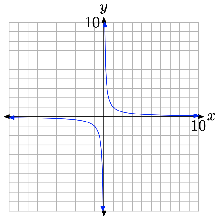
The complete graph of y = 1/x in Figure \(\PageIndex{5}\) is called a hyperbola and serves as a fundamental starting point for all subsequent discussion in this section.
We noted earlier that the domain of the function defined by the equation y = 1/x is the set \(D=\{x : x \neq 0\}\). Zero is excluded from the domain because division by zero is undefined. It’s no coincidence that the graph has a vertical asymptote at x = 0. We’ll see this relationship reinforced in further examples.
Translations
In this section, we will translate the graph of y = 1/x in both the horizontal and vertical directions.
Sketch the graph of
\[y=\frac{1}{x+3}-4 \nonumber \]
Solution
Technically, the function defined by y = 1/(x + 3) − 4 does not have the general form (3) of a rational function. However, in later chapters we will show how y = 1/(x + 3) − 4 can be manipulated into the general form of a rational function.
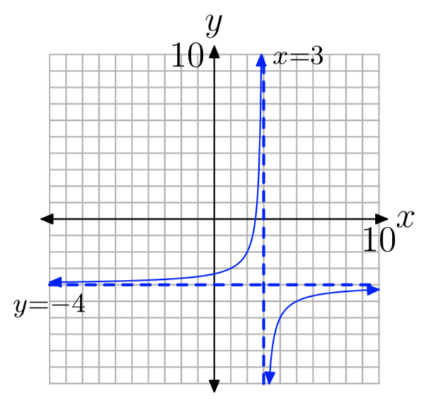
We know what the graph of y = 1/x looks like. If we replace x with x + 3, this will shift the graph of y = 1/x three units to the left, as shown in Figure \(\PageIndex{6}\)(a). Note that the vertical asymptote has also shifted 3 units to the left of its original position (the y-axis) and now has equation x = −3. By tradition, we draw the vertical asymptote as a dashed line.
If we subtract 4 from the result in Figure \(\PageIndex{6}\)(a), this will shift the graph in Figure \(\PageIndex{6}\)(a) four units downward to produce the graph shown in Figure \(\PageIndex{6}\)(b). Note that the horizontal asymptote also shifted 4 units downward from its original position (the x-axis) and now has equation y = −4.
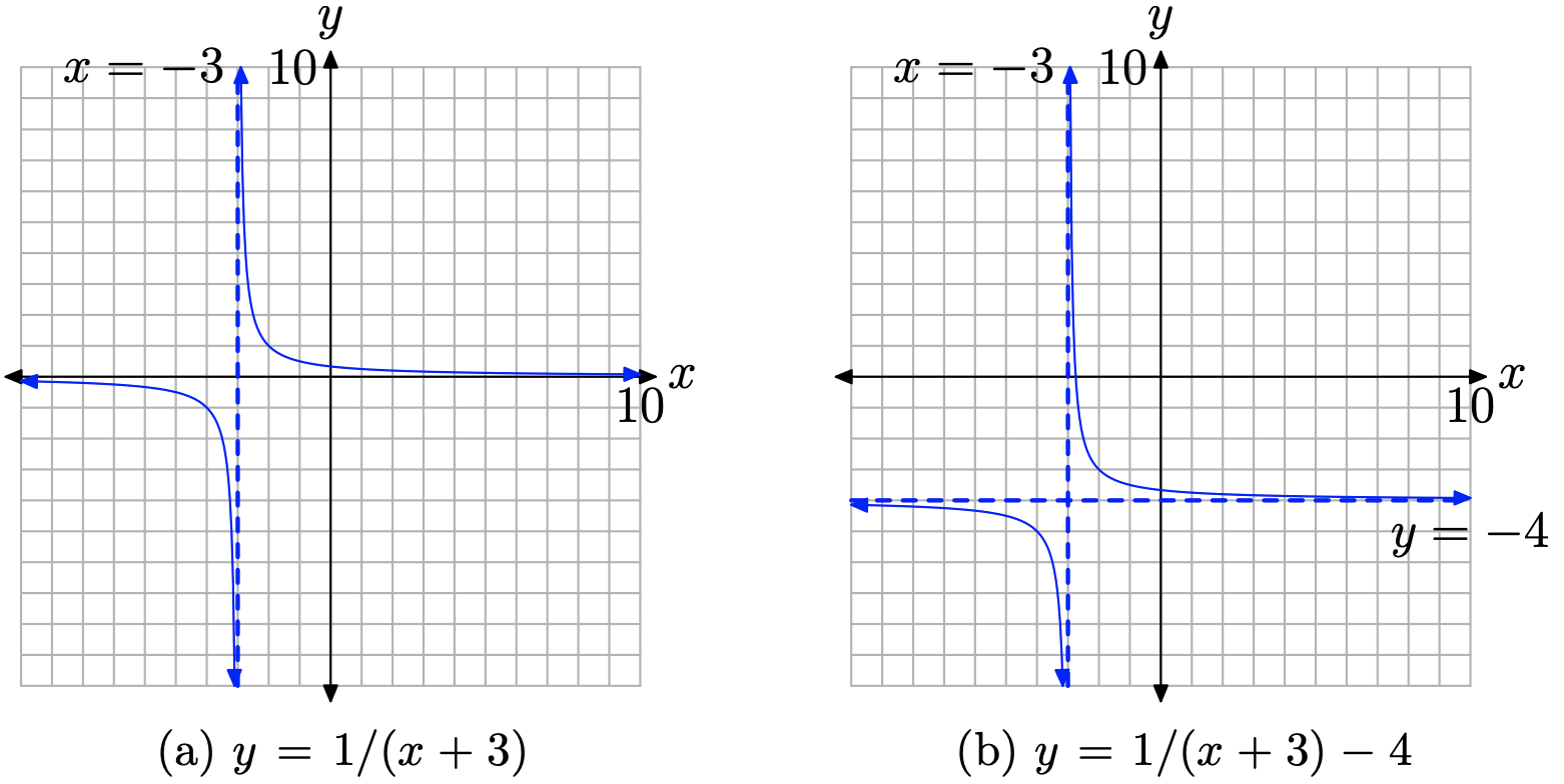
If you examine equation (11), you note that you cannot use x = −3 as this will make the denominator of equation (11) equal to zero. In Figure \(\PageIndex{6}\)(b), note that there is a vertical asymptote in the graph of equation (11) at x = −3. This is a common occurrence, which will be a central theme of this chapter.
Let’s ask another key question.
What are the domain and range of the rational function presented in Example \(\PageIndex{1}\)?
Solution
You can glance at the equation
\[y=\frac{1}{x+3}-4\nonumber \]
of Example \(\PageIndex{1}\) and note that x = −3 makes the denominator zero and must be excluded from the domain. Hence, the domain of this function is \(D=\{x : x \neq-3\}\).
However, you can also determine the domain by examining the graph of the function in Figure \(\PageIndex{6}\)(b). Note that the graph extends indefinitely to the left and right. One might first guess that the domain is all real numbers if it were not for the vertical asymptote at x = −3 interrupting the continuity of the graph. Because the graph of the function gets arbitrarily close to this vertical asymptote (on either side) without actually touching the asymptote, the graph does not contain a point having an x-value equaling −3. Hence, the domain is as above, \(D=\{x : x \neq-3\}\). This is comforting that the graphical analysis agrees with our earlier analytical determination of the domain.
The graph is especially helpful in determining the range of the function. Note that the graph rises to positive infinity and falls to negative infinity. One would first guess that the range is all real numbers if it were not for the horizontal asymptote at y = −4 interrupting the continuity of the graph. Because the graph gets arbitrarily close to the horizontal asymptote (on either side) without actually touching the asymptote, the graph does not contain a point having a y-value equaling −4. Hence, −4 is excluded from the range. That is, \(R=\{y : y \neq-4\}\).
Scaling and Reflection
In this section, we will both scale and reflect the graph of y = 1/x. For extra measure, we also throw in translations in the horizontal and vertical directions.
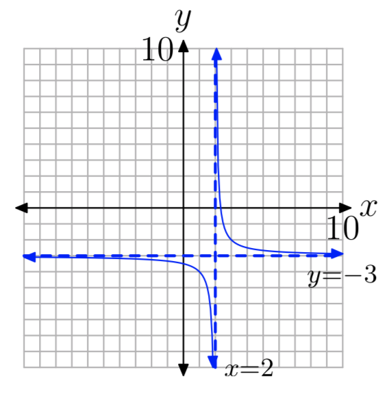
Sketch the graph of \[y=-\frac{2}{x-4}+3\nonumber \]
Solution
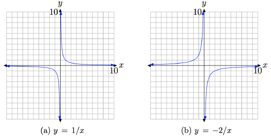
First, we multiply the equation y = 1/x by −2 to get
\[y=-\frac{2}{x}\nonumber \]
Multiplying by 2 should stretch the graph in the vertical directions (both positive and negative) by a factor of 2. Note that points that are very near the x-axis, when doubled, are not going to stray too far from the x-axis, so the horizontal asymptote will remain the same. Finally, multiplying by −2 will not only stretch the graph, it will also reflect the graph across the x-axis, as shown in Figure \(\PageIndex{7}\)(b).
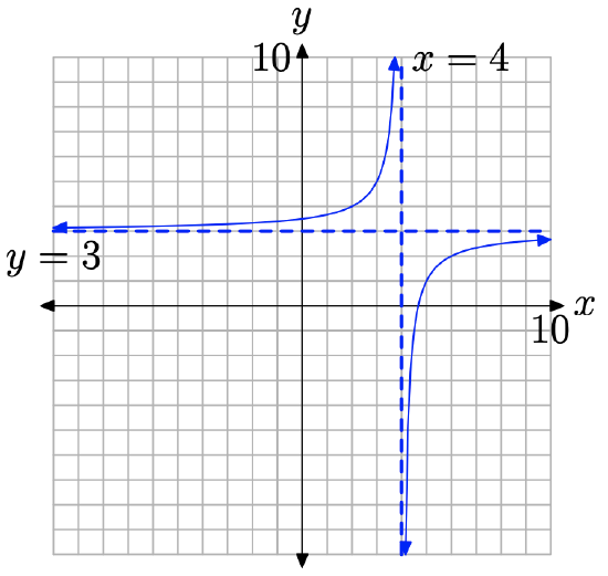
Replacing x with x − 4 will shift the graph 4 units to the right, then adding 3 will shift the graph 3 units up, as shown in Figure \(\PageIndex{8}\). Note again that x = 4 makes the denominator of y = −2/(x − 4) + 3 equal to zero and there is a vertical asymptote at x = 4. The domain of this function is \(D=\{x : x \neq 4\}\).
As x approaches positive or negative infinity, points on the graph of y = −2/(x−4)+ 3 get arbitrarily close to the horizontal asymptote y = 3 but never touch it. Therefore, there is no point on the graph that has a y-value of 3. Thus, the range of the function is the set \(R=\{y : y \neq 3\}\).
Difficulties with the Graphing Calculator
The graphing calculator does a very good job drawing the graphs of “continuous functions.”
A continuous function is one that can be drawn in one continuous stroke, never lifting pen or pencil from the paper during the drawing.
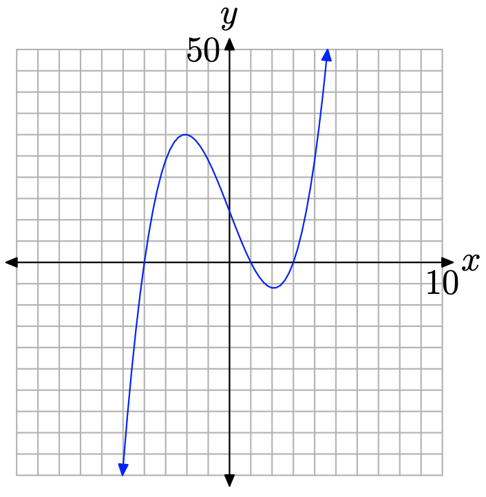
Polynomials, such as the one in Figure \(\PageIndex{9}\), are continuous functions.
Unfortunately, a rational function with vertical asymptote(s) is not a continuous function. First, you have to lift your pen at points where the denominator is zero, because the function is undefined at these points. Secondly, it’s not uncommon to have to jump from positive infinity to negative infinity (or vice-versa) when crossing a vertical asymptote. When this happens, we have to lift our pen and shift it before continuing with our drawing.
However, the graphing calculator does not know how to do this “lifting” of the pen near vertical asymptotes. The graphing calculator only knows one technique, plot a point, then connect it with a segment to the last point plotted, move an incremental distance and repeat. Consequently, when the graphing calculator crosses a vertical asymptote where there is a shift from one type of infinity to another (e.g., from positive to negative), the calculator draws a “false line” of connection, one that it should not draw. Let’s demonstrate this aberration with an example.
Use a graphing calculator to draw the graph of the rational function in Example \(\PageIndex{3}\).
Solution
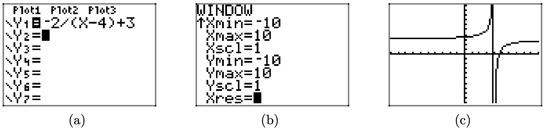
Load the equation into your calculator, as shown in Figure \(\PageIndex{10}\)(a). Set the window as shown in Figure \(\PageIndex{10}\)(b), then push the GRAPH button to draw the graph shown in Figure \(\PageIndex{10}\)(c). Results may differ on some calculators, but in our case, note the “false line” drawn from the top of the screen to the bottom, attempting to “connect” the two branches of the hyperbola.
Some might rejoice and claim, “Hey, my graphing calculator draws vertical asymptotes.” However, before you get too excited, note that in Figure \(\PageIndex{8}\) the vertical asymptote should occur at exactly x = 4. If you look very carefully at the “vertical line” in Figure \(\PageIndex{10}\)(c), you’ll note that it just misses the tick mark at x = 4. This “vertical line” is a line that the calculator should not draw. The calculator is attempting to draw a continuous function where one doesn’t exist.
One possible workaround is to press the MODE button on your keyboard, which opens the menu shown in Figure \(\PageIndex{11}\)(a). Use the arrow keys to highlight DOT instead of CONNECTED and press the ENTER key to make the selection permanent. Press the GRAPH button to draw the graph in Figure \(\PageIndex{11}\)(b).
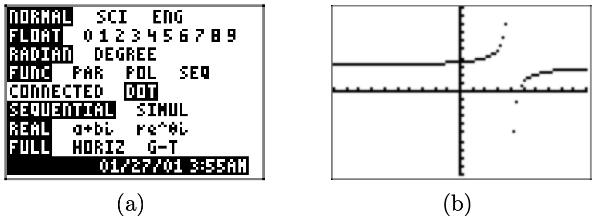
This “dot mode” on your calculator calculates the next point on the graph and plots the point, but it does not connect it with a line segment to the previously plotted point. This mode is useful in demonstrating that the vertical line in Figure \(\PageIndex{10}\)(c) is not really part of the graph, but we lose some parts of the graph we’d really like to see. Compromise is in order.
This example clearly shows that intelligent use of the calculator is a required component of this course. The calculator is not simply a “black box” that automatically does what you want it to do. In particular, when you are drawing rational functions, it helps to know ahead of time the placement of the vertical asymptotes. Knowledge of the asymptotes, coupled with what you see on your calculator screen, should enable you to draw a graph as accurate as that shown in Figure \(\PageIndex{8}\).
Gentle reminder. You’ll want to set your calculator back in “connected mode.” To do this, press the MODE button on your keyboard to open the menu in Figure \(\PageIndex{10}\)(a) once again. Use your arrow keys to highlight CONNECTED, then press the ENTER key to make the selection permanent.
Exercise
In Exercises 1-14, perform each of the following tasks for the given rational function.
- Set up a coordinate system on a sheet of graph paper. Label and scale each axis.
- Use geometric transformations as in Examples 10, 12, and 13 to draw the graphs of each of the following rational functions. Draw the vertical and horizontal asymptotes as dashed lines and label each with its equation. You may use your calculator to check your solution, but you should be able to draw the rational function without the use of a calculator.
- Use set-builder notation to describe the domain and range of the given rational function.
\(f(x) = −\frac{2}{x}\)
- Answer
-
D = {x: \(x \ne 0\)}, R = {y: \(y \ne 0\)}
\(f(x) = \frac{3}{x}\)
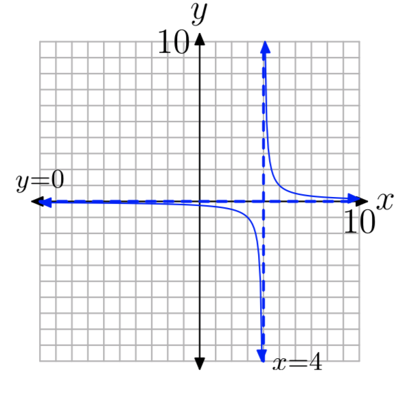
\(f(x) = \frac{1}{x−4}\)
- Answer
-
D = {x: \(x \ne 4\)}, R = {y: \(y \ne 0\)}
\(f(x) = \frac{1}{x+3}\)
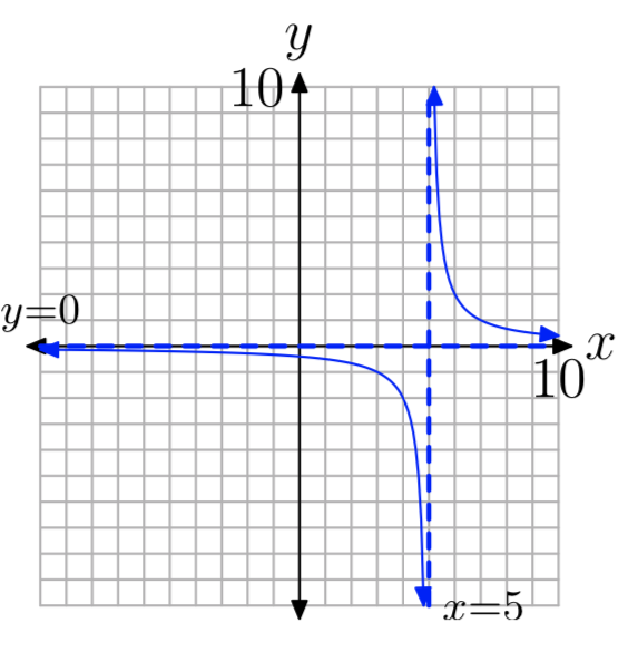
\(f(x) = \frac{2}{x−5}\)
- Answer
-
D = {x: \(x \ne 5\)}, R = {y: \(y \ne 0\)}
\(f(x) = −\frac{3}{x+6}\)
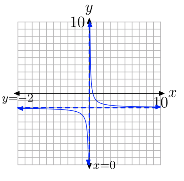
\(f(x) = \frac{1}{x}−2\)
- Answer
-
D = {x: \(x \ne 0\)}, R = {y: \(y \ne −2\)}
\(f(x) = −\frac{1}{x}+4\)
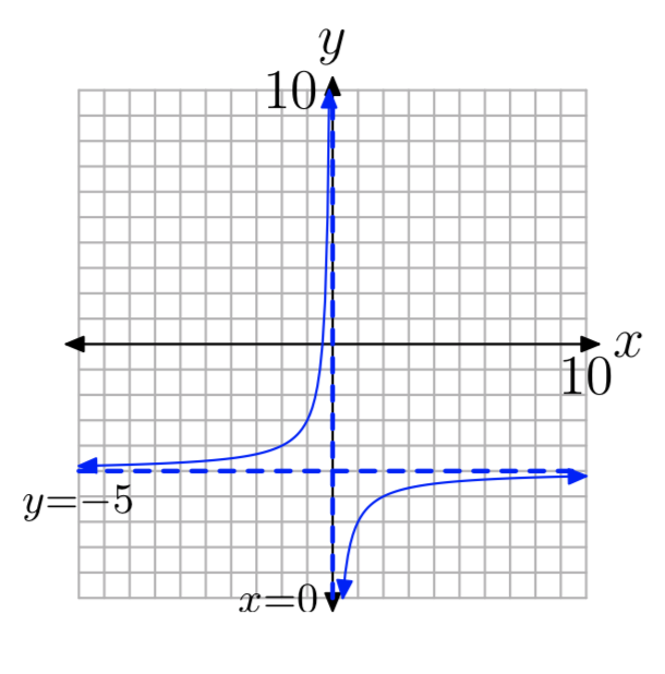
\(f(x) = −\frac{2}{x}−5\)
- Answer
-
D = {x: \(x \ne 0\)}, R = {y: \(y \ne −5\)}
\(f(x) = \frac{3}{x}−5\)
\(f(x) = \frac{1}{x−2}−3\)
- Answer
-
D = {x: \(x \ne 2\)}, R = {y: \(y \ne −3\)}
\(f(x) = −\frac{1}{x+1}+5\)
\(f(x) = −\frac{2}{x−3}−4\)
- Answer
-
D = {x: \(x \ne 3\)}, R = {y: \(y \ne −4\)}
\(f(x) = \frac{3}{x+5}−2\)
In Exercises 15-22, find all vertical asymptotes, if any, of the graph of the given function.
\(f(x) = −\frac{5}{x+1}−3\)
- Answer
-
Vertical asymptote: x = −1
\(f(x) = \frac{6}{x+8}+2\)
\(f(x) = −\frac{9}{x+2}−6\)
- Answer
-
Vertical asymptote: x = −2
\(f(x) = −\frac{8}{x−4}−5\)
\(f(x) = \frac{2}{x+5}+1\)
- Answer
-
Vertical asymptote: x = −5
\(f(x) = −\frac{3}{x+9}+2\)
\(f(x) = \frac{7}{x+8}−9\)
- Answer
-
Vertical asymptote: x = −8
\(f(x) = \frac{6}{x−5}−8\)
In Exercises 23-30, find all horizontal asymptotes, if any, of the graph of the given function.
\(f(x) = \frac{5}{x+7}+9\)
- Answer
-
Horizontal asymptote: y = 9
\(f(x) = −\frac{8}{x+7}−4\)
\(f(x) = \frac{8}{x+5}−1\)
- Answer
- Horizontal asymptote: y = −1
\(f(x) = −\frac{2}{x+3}+8\)
\(f(x) = \frac{7}{x+1}−9\)
- Answer
-
Horizontal asymptote: y = −9
\(f(x) = −\frac{2}{x−1}+5\)
\(f(x) = \frac{5}{x+2}−4\)
- Answer
-
Horizontal asymptote: y = −4
\(f(x) = −\frac{6}{x−1}−2\)
In Exercises 31-38, state the domain of the given rational function using set-builder notation.
\(f(x) = −\frac{4}{x+5}+5\)
- Answer
-
Domain = {x: \(x \ne −5\)}
\(f(x) = −\frac{7}{x−6}+1\)
\(f(x) = \frac{6}{x−5}+1\)
- Answer
-
Domain = {x: \(x \ne 5\)}
\(f(x) = −\frac{5}{x−3}−9\)
\(f(x) = \frac{1}{x+7}+2\)
- Answer
-
Domain = {x: \(x \ne −7\)}
\(f(x) = −\frac{2}{x−5}+4\)
\(f(x) = −\frac{4}{x+2}+2\)
- Answer
-
Domain = {x: \(x \ne −2\)}
\(f(x) = \frac{2}{x+6}+9\)
In Exercises 39-46, find the range of the given function, and express your answer in set notation.
\(f(x) = \frac{2}{x−3}+8\)
- Answer
-
Range = {y: \(y \ne 8\)}
\(f(x) = \frac{4}{x−3}+5\)
\(f(x) = −\frac{5}{x−8}−5\)
- Answer
-
Range = {y: \(y \ne −5\)}
\(f(x) = −\frac{2}{x+1}+6\)
\(f(x) = \frac{7}{x+7}+5\)
- Answer
-
Range = {y: \(y \ne 5\)}
\(f(x) = −\frac{8}{x+3}+9\)
\(f(x) = \frac{4}{x+3}−2\)
- Answer
-
Range = {y: \(y \ne −2\)}
\(f(x) = −\frac{5}{x−4}+9\)