
4.1: System of Equations - Graphing


( \newcommand{\kernel}{\mathrm{null}\,}\)
Given two linear equations and after graphing the lines,
Solution 1. If the two lines intersect, then the point of intersection is the solution to the system, i.e., the solution is an ordered-pair (x,y).
Solution 2. If the two lines do not intersect and are parallel, i.e., they have the same slope and different y-intercepts, then the system has no solution.
Solution 3. If the two lines are the same line, then the solution is infinitely many solutions on that line.
Verifying Solutions
Is the ordered-pair (2,1) a solution to the system {3x−y=5x+y=3?
Solution
To verify whether (2,1) is the solution to the system, we plug-n-chug (2,1) into each equation and determine whether we obtain a true statement. If we obtain true statements for both equations in the system, then (2,1) will be the solution to the system.
3x−y=5Plug-n-chug x=2 and y=13(2)−(1)?=5Simplify6−1?=5Subtract5=5✓True
Let’s do the same for the second equation:
x+y=3Plug-n-chug x=2 and y=1(2)+(1)?=3Add3=3✓True
Since the ordered-pair (2,1) makes both statements true, then (2,1) is a solution to the system. Hence, if we were to graph these lines, they would intersect at the point (2,1).
Is the ordered-pair (−3,−4) a solution to the system {5x+4y=−313x+6y=−36?
Solution
To verify whether (−3,−4) is the solution to the system, we plug-n-chug (−3,−4) into each equation and determine whether we obtain a true statement. If we obtain true statements for both equations in the system, then (−3,−4) will be the solution to the system.
5x+4y=−31Plug-n-chug x=−3 and y=−45(−3)+4(−4)?=−31Simplify−15−16?==31Subtract−31=−31✓True
Let’s do the same for the second equation:
3x+6y=−36Plug-n-chug x=−3 and y=−43(−3)+6(−4)?=−36Simplify−9−24?=−36Subtract−33≠−36XFalse
Since the ordered-pair (−3,−4) makes only one of the statements true, then (−3,−4) is not a solution to the system. Recall, the ordered-pair must make the statement true for both equations in order to be a solution to the system.
Solve a System by Graphing
Solve the system by graphing: {y=−12x+3y=34x−2
Solution
We first need to decide the method in which we will graph. We learned in the previous chapter to make a table, use intercepts, or use the slope-intercept form. Notice both equations are given in slope-intercept form. Let’s go ahead and use the slope-intercept form to graph the lines.
y=−12x+3(1)y=34x−2(2)
We will graph line (1) with a solid line and graph line (2) with a dashed line.
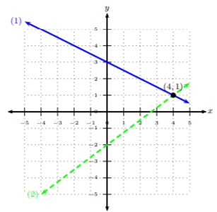
We can see after graphing the two lines that they intersect at the point (4,1). Hence, the solution to the system is (4,1).
Solve the system by graphing: {6x−3y=−92x+2y=−6
Solution
We first need to decide the method in which we will graph. We learned in the previous chapter to make a table, use intercepts, or use the slope-intercept form. Since both equations are not given in slope-intercept form as in Example 4.1.3 , we can rewrite them in slope-intercept form, then graph. So, let’s rewrite each equation in slope-intercept form: 6x−3y=−92x+2y=−6−3y=−6x−92y=−2x−6y=−6x−3−9−3y=−22x−62y=2x+3y=−x−3
Let’s go ahead and use the slope-intercept form to graph the lines.
y=2x+3(1)y=−x−3(2)
We will graph line (1) with a solid line and graph line (2) with a dashed line.
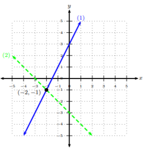
We can see after graphing the two lines that they intersect at the point (−2,−1). Hence, the solution to the system is (−2,−1).
Solve the system by graphing: {y=32x−4y=32x+1
Solution
We first need to decide the method in which we will graph. We learned in the previous chapter to make a table, use intercepts, or use the slope-intercept form. Notice both equations are given in slope-intercept form. Let’s go ahead and use the slope-intercept form to graph the lines.
y=32x−4(1)y=32x+1(2)
We will graph line (1) with a solid line and graph line (2) with a dashed line.
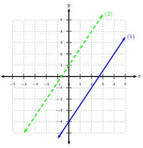
We can see after graphing the two lines that these two lines are parallel. Hence, there is no solution to the system (since they will never intersect). Note, we could see by the system that these lines shared the same slope, but had different y-intercepts. Without graphing, we could have seen that these lines were parallel, hence, having no solution.
Solve the system by graphing: {2x−6y=123x−9y=18
Solution
We first need to decide the method in which we will graph. We learned in the previous chapter to make a table, use intercepts, or use the slope-intercept form. Since neither of the equations are written in slope-intercept form, let’s try graphing by making a table for each equation. Start with equation (1):
x=−32(−3)−6y=12−6−6y=12−6y=18y=−3
x=02(0)−6y=12−6y=12y=−2
x=32(3)−6y=126−6y=12−6y=6y=−1
| x | y |
|---|---|
| −3 | −3 |
| 0 | −2 |
| 3 | −1 |
Next, equation (2):
x=−33(−3)−9y=18−9−9y=18−9y=27y=−3
x=03(0)−9y=18−9y=18y=−2
x=33(3)−9y=189−9y=18−9y=9y=−1
| x | y |
|---|---|
| −3 | −3 |
| 0 | −2 |
| 3 | −1 |
Now, let’s graph the ordered-pairs. We will graph line (1) with a solid line and graph line (2) with a dashed line.
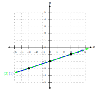
We can see after graphing the two lines that these two lines are the same. Hence, there are infinitely many solutions on the line 2x−6y=12 (or the other equation) to the system (since they intersect at every point on the line). Note, we could see by the system that these lines shared the same slope and y-intercepts (after putting them in slope-intercept form). Without graphing, we could have seen that these lines were the same line, hence, having infinitely many solutions.
The Babylonians were the first to work with systems of equations with two variables. However, their work with systems was quickly passed by the Greeks, around 300 AD, who would solve systems of equations with three or four variables and eventually developed methods for solving systems with any number of unknowns.
Systems of Equations: Graphing Homework
Determine whether the given ordered pair(s) is a solution to the system.
2x+8y=0−8x+3y=38;(−4,1)
−5x+6y=114x+2y=−4;(−1,1)
6x+5y=49−x−6y=−34;(4,5)
−2x+2y=−8−6x−3y=−6;(2,−2)
Solve each system by graphing.
y=−x+1y=−5x−3
y=−3y=−x−4
y=−34x+1y=−34x+2
y=13x+2y=−53x−4
y=53x+4y=−23x−3
x+3y=−95x+3y=3
x−y=42x+y=−1
2x+3y=−62x+y=2
2x+y=2x−y=4
2x+y=−2x+3y=9
0=−6x−9y+3612=6x−3y
2x−y=−10=−2x−y−3
3+y=−x−4−6x=−y
−y+7x=4−y−3+7x=0
−12+x=4y12−5x=4y
y=−54x−2y=−14x+2
y=−x−2y=23x+3
y=2x+2y=−x−4
y=2x−4y=12x+2
y=12x+4y=12x+1
x+4y=−122x+y=4
6x+y=−3x+y=2
3x+2y=23x+2y=−6
x+2y=65x−4y=16
x−y=35x+2y=8
−2y+x=42=−x+12y
−2y=−4−x−2y=−5x+4
16=−x−4y−2x=−4−4y
−4+y=xx+2=−y
−5x+1=−y−y+x=−3