
8.4: Integration of Elementary Functions
- Page ID
- 19214

\( \newcommand{\vecs}[1]{\overset { \scriptstyle \rightharpoonup} {\mathbf{#1}} } \)
\( \newcommand{\vecd}[1]{\overset{-\!-\!\rightharpoonup}{\vphantom{a}\smash {#1}}} \)
\( \newcommand{\dsum}{\displaystyle\sum\limits} \)
\( \newcommand{\dint}{\displaystyle\int\limits} \)
\( \newcommand{\dlim}{\displaystyle\lim\limits} \)
\( \newcommand{\id}{\mathrm{id}}\) \( \newcommand{\Span}{\mathrm{span}}\)
( \newcommand{\kernel}{\mathrm{null}\,}\) \( \newcommand{\range}{\mathrm{range}\,}\)
\( \newcommand{\RealPart}{\mathrm{Re}}\) \( \newcommand{\ImaginaryPart}{\mathrm{Im}}\)
\( \newcommand{\Argument}{\mathrm{Arg}}\) \( \newcommand{\norm}[1]{\| #1 \|}\)
\( \newcommand{\inner}[2]{\langle #1, #2 \rangle}\)
\( \newcommand{\Span}{\mathrm{span}}\)
\( \newcommand{\id}{\mathrm{id}}\)
\( \newcommand{\Span}{\mathrm{span}}\)
\( \newcommand{\kernel}{\mathrm{null}\,}\)
\( \newcommand{\range}{\mathrm{range}\,}\)
\( \newcommand{\RealPart}{\mathrm{Re}}\)
\( \newcommand{\ImaginaryPart}{\mathrm{Im}}\)
\( \newcommand{\Argument}{\mathrm{Arg}}\)
\( \newcommand{\norm}[1]{\| #1 \|}\)
\( \newcommand{\inner}[2]{\langle #1, #2 \rangle}\)
\( \newcommand{\Span}{\mathrm{span}}\) \( \newcommand{\AA}{\unicode[.8,0]{x212B}}\)
\( \newcommand{\vectorA}[1]{\vec{#1}} % arrow\)
\( \newcommand{\vectorAt}[1]{\vec{\text{#1}}} % arrow\)
\( \newcommand{\vectorB}[1]{\overset { \scriptstyle \rightharpoonup} {\mathbf{#1}} } \)
\( \newcommand{\vectorC}[1]{\textbf{#1}} \)
\( \newcommand{\vectorD}[1]{\overrightarrow{#1}} \)
\( \newcommand{\vectorDt}[1]{\overrightarrow{\text{#1}}} \)
\( \newcommand{\vectE}[1]{\overset{-\!-\!\rightharpoonup}{\vphantom{a}\smash{\mathbf {#1}}}} \)
\( \newcommand{\vecs}[1]{\overset { \scriptstyle \rightharpoonup} {\mathbf{#1}} } \)
\(\newcommand{\longvect}{\overrightarrow}\)
\( \newcommand{\vecd}[1]{\overset{-\!-\!\rightharpoonup}{\vphantom{a}\smash {#1}}} \)
\(\newcommand{\avec}{\mathbf a}\) \(\newcommand{\bvec}{\mathbf b}\) \(\newcommand{\cvec}{\mathbf c}\) \(\newcommand{\dvec}{\mathbf d}\) \(\newcommand{\dtil}{\widetilde{\mathbf d}}\) \(\newcommand{\evec}{\mathbf e}\) \(\newcommand{\fvec}{\mathbf f}\) \(\newcommand{\nvec}{\mathbf n}\) \(\newcommand{\pvec}{\mathbf p}\) \(\newcommand{\qvec}{\mathbf q}\) \(\newcommand{\svec}{\mathbf s}\) \(\newcommand{\tvec}{\mathbf t}\) \(\newcommand{\uvec}{\mathbf u}\) \(\newcommand{\vvec}{\mathbf v}\) \(\newcommand{\wvec}{\mathbf w}\) \(\newcommand{\xvec}{\mathbf x}\) \(\newcommand{\yvec}{\mathbf y}\) \(\newcommand{\zvec}{\mathbf z}\) \(\newcommand{\rvec}{\mathbf r}\) \(\newcommand{\mvec}{\mathbf m}\) \(\newcommand{\zerovec}{\mathbf 0}\) \(\newcommand{\onevec}{\mathbf 1}\) \(\newcommand{\real}{\mathbb R}\) \(\newcommand{\twovec}[2]{\left[\begin{array}{r}#1 \\ #2 \end{array}\right]}\) \(\newcommand{\ctwovec}[2]{\left[\begin{array}{c}#1 \\ #2 \end{array}\right]}\) \(\newcommand{\threevec}[3]{\left[\begin{array}{r}#1 \\ #2 \\ #3 \end{array}\right]}\) \(\newcommand{\cthreevec}[3]{\left[\begin{array}{c}#1 \\ #2 \\ #3 \end{array}\right]}\) \(\newcommand{\fourvec}[4]{\left[\begin{array}{r}#1 \\ #2 \\ #3 \\ #4 \end{array}\right]}\) \(\newcommand{\cfourvec}[4]{\left[\begin{array}{c}#1 \\ #2 \\ #3 \\ #4 \end{array}\right]}\) \(\newcommand{\fivevec}[5]{\left[\begin{array}{r}#1 \\ #2 \\ #3 \\ #4 \\ #5 \\ \end{array}\right]}\) \(\newcommand{\cfivevec}[5]{\left[\begin{array}{c}#1 \\ #2 \\ #3 \\ #4 \\ #5 \\ \end{array}\right]}\) \(\newcommand{\mattwo}[4]{\left[\begin{array}{rr}#1 \amp #2 \\ #3 \amp #4 \\ \end{array}\right]}\) \(\newcommand{\laspan}[1]{\text{Span}\{#1\}}\) \(\newcommand{\bcal}{\cal B}\) \(\newcommand{\ccal}{\cal C}\) \(\newcommand{\scal}{\cal S}\) \(\newcommand{\wcal}{\cal W}\) \(\newcommand{\ecal}{\cal E}\) \(\newcommand{\coords}[2]{\left\{#1\right\}_{#2}}\) \(\newcommand{\gray}[1]{\color{gray}{#1}}\) \(\newcommand{\lgray}[1]{\color{lightgray}{#1}}\) \(\newcommand{\rank}{\operatorname{rank}}\) \(\newcommand{\row}{\text{Row}}\) \(\newcommand{\col}{\text{Col}}\) \(\renewcommand{\row}{\text{Row}}\) \(\newcommand{\nul}{\text{Nul}}\) \(\newcommand{\var}{\text{Var}}\) \(\newcommand{\corr}{\text{corr}}\) \(\newcommand{\len}[1]{\left|#1\right|}\) \(\newcommand{\bbar}{\overline{\bvec}}\) \(\newcommand{\bhat}{\widehat{\bvec}}\) \(\newcommand{\bperp}{\bvec^\perp}\) \(\newcommand{\xhat}{\widehat{\xvec}}\) \(\newcommand{\vhat}{\widehat{\vvec}}\) \(\newcommand{\uhat}{\widehat{\uvec}}\) \(\newcommand{\what}{\widehat{\wvec}}\) \(\newcommand{\Sighat}{\widehat{\Sigma}}\) \(\newcommand{\lt}{<}\) \(\newcommand{\gt}{>}\) \(\newcommand{\amp}{&}\) \(\definecolor{fillinmathshade}{gray}{0.9}\)In Chapter 5, integration was treated as antidifferentiation. Now we adopt another, measure-theoretical approach.
Lebesgue's original theory was based on Lebesgue measure (Chapter 7, §8). The more general modern treatment develops the integral for functions \(f : S \rightarrow E\) in an arbitrary measure space. Henceforth, \((S, \mathcal{M}, m)\) is fixed, and the range space \(E\) is \(E^{1}, E^{*}, C, E^{n},\) or another complete normed space. Recall that in such a space, \(\sum_{i}\left|a_{i}\right|<\infty\) implies that \(\sum a_{i}\) converges and is permutable (Chapter 7, §2).
We start with elementary maps, including simple maps as a special case.
Let \(f : S \rightarrow E\) be elementary on \(A \in \mathcal{M};\) so \(f=a_{i}\) on \(A_{i}\) for some \(\mathcal{M}\)-partition
\[A=\bigcup_{i} A_{i} \text { (disjoint).}\]
(Note that there may be many such partitions.)
We say that \(f\) is integrable (with respect to \(m\)), or \(m\)-integrable, on \(A\) iff
\[\sum\left|a_{i}\right| m A_{i}<\infty.\]
(The notation "\(|a_{i}| m A_{i}\)" always makes sense by our conventions (2*) in Chapter 4, §4.) If \(m\) is Lebesgue measure, then we say that \(f\) is Lebesgue integrable, or L-integrable.
We then define \(\int_{A} f,\) the \(m\)-integral of \(f\) on \(A,\) by
\[\int_{A} f=\int_{A} f d m=\sum_{i} a_{i} m A_{i}.\]
(The notation "\(dm\)" is used to specify the measure \(m\).)
The "classical" notation for \(\int_{A} f d m\) is \(\int_{A} f(x) d m(x)\).
Note 1. The assumption
\[\sum\left|a_{i}\right| m A_{i}<\infty\]
implies
\[(\forall i) \quad\left|a_{i}\right| m A_{i}<\infty;\]
so \(a_{i}=0\) if \(m A_{i}=\infty,\) and \(m A_{i}=0\) if \(|a_{i}|=\infty.\) Thus by our conventions, all "bad" terms \(a_{i} m A_{i}\) vanish. Hence the sum in (1) makes sense and is finite.
Note 2. This sum is also independent of the particular choice of \(\{A_{i}\}.\) For if \(\{B_{k}\}\) is another \(\mathcal{M}\)-partition of \(A,\) with \(f=b_{k}\) on \(B_{k},\) say, then \(f=a_{i}=b_{k}\) on \(A_{i} \cap B_{k}\) whenever \(A_{i} \cap B_{k} \neq \emptyset.\) Also,
\[(\forall i) \quad A_{i}=\bigcup_{k}\left(A_{i} \cap B_{k}\right) \text { (disjoint);}\]
so
\[(\forall i) \quad a_{i} m A_{i}=\sum_{k} a_{i} m(A_{i} \cap B_{k}),\]
and hence (see Theorem 2 of Chapter 7, §2, and Problem 11 there)
\[\sum_{i} a_{i} m A_{i}=\sum_{i} \sum_{k} a_{i} m\left(A_{i} \cap B_{k}\right)=\sum_{k} \sum_{i} b_{k} m\left(A_{i} \cap B_{k}\right)=\sum_{k} b_{k} m B_{k}.\]
(Explain!)
This makes our definition (1) unambiguous and allows us to choose any \(\mathcal{M}\)-partition \(\{A_{i}\},\) with \(f\) constant on each \(A_{i},\) when forming integrals (1).
Let \(f : S \rightarrow E\) be elementary and integrable on \(A \in \mathcal{M}.\) Then the following statements are true.
(i) \(|f|<\infty\) a.e. on \(A.\)
(ii) \(f\) and \(|f|\) are elementary and integrable on any \(\mathcal{M}\)-set \(B \subseteq A,\) and
\[\left|\int_{B} f\right| \leq \int_{B}|f| \leq \int_{A}|f|.\]
(iii) The set \(B=A(f \neq 0)\) is \(\sigma\)-finite (Definition 4 in Chapter 7, §5), and
\[\int_{A} f=\int_{B} f.\]
(iv) If \(f=a\) (constant) on \(A\),
\[\int_{A} f=a \cdot m A.\]
(v) \(\int_{A}|f|=0\) iff \(f=0\) a.e. on \(A\).
(vi) If \(m Q=0,\) then
\[\int_{A} f=\int_{A-Q} f\]
(so we may neglect sets of measure 0 in integrals).
(vii) For any \(k\) in the scalar field of \(E, k f\) is elementary and integrable, and
\[\int_{A} k f=k \int_{A} f.\]
Note that if \(f\) is scalar valued, \(k\) may be a vector. If \(E=E^{*},\) we assume \(k \in E^{1}.\)
- Proof
-
(i) By Note 1, \(|f|=|a_{i}|=\infty\) only on those \(A_{i}\) with \(m A_{i}=0.\) Let \(Q\) be the union of all such \(A_{i}.\) Then \(m Q=0\) and \(|f|<\infty\) on \(A-Q,\) proving (i).
(ii) If \(\{A_{i}\}\) is an \(\mathcal{M}\)-partition of \(A,\{B \cap A_{i}\}\) is one for \(B.\) (Verify!) We have \(f=a_{i}\) and \(|f|=|a_{i}|\) on \(B \cap A_{i} \subseteq A_{i}\).
Also,
\[\sum\left|a_{i}\right| m\left(B \cap A_{i}\right) \leq \sum\left|a_{i}\right| m A_{i}<\infty.\]
(Why?) Thus \(f\) and \(|f|\) are elementary and integrable on \(B,\) and (ii) easily follows by formula (1).
(iii) By Note 1, \(f=0\) on \(A_{i}\) if \(m A_{i}=\infty.\) Thus \(f \neq 0\) on \(A_{i}\) only if \(m A_{i}<\infty\). Let \(\{A_{i_{k}}\}\) be the subsequence of those \(A_{i}\) on which \(f \neq 0;\) so
\[(\forall k) \quad m A_{i_{k}}<\infty.\]
Also,
\[B=A(f \neq 0)=\bigcup_{k} A_{i_{k}} \in \mathcal{M} \text{ (}\sigma \text {-finite!).}\]
By (ii), \(f\) is elementary and integrable on \(B.\) Also,
\[\int_{B} f=\sum_{k} a_{i_{k}} m A_{i_{k}},\]
while
\[\int_{A} f=\sum_{i} a_{i} m A_{i}.\]
These sums differ only by terms with \(a_{i}=0.\) Thus (iii) follows.
The proof of (iv)-(vii) is left to the reader.\(\quad \square\)
Note 3. If \(f : S \rightarrow E^{*}\) is elementary and sign-constant on \(A,\) we also allow that
\[\int_{A} f=\sum_{i} a_{i} m A_{i}=\pm \infty.\]
Thus here \(\int_{A} f\) exists even if \(f\) is not integrable. Apart from claims of integrability and \(\sigma\)-finiteness, Corollary 1(ii)-(vii) hold for such \(f\), with the same proofs.
Let \(m\) be Lebesgue measure in \(E^{1}.\) Define \(f=1\) on \(R\) (rationals) and \(f=0\) on \(E^{1}-R ;\) see Chapter 4, §1, Example (c). Let \(A=[0,1].\)
By Corollary 1 in Chapter 7, §8, \(A \cap R \in \mathcal{M}^{*}\) and \(m(A \cap R)=0.\) Also, \(A-R \in \mathcal{M}^{*}\).
Thus \(\{A \cap R, A-R\}\) is an \(\mathcal{M}^{*}\)-partition of \(A,\) with \(f=1\) on \(A \cap R\) and \(f=0\) on \(A-R.\)
Hence \(f\) is elementary and integrable on \(A,\) and
\[\int_{A} f=1 \cdot m(A \cap R)+0 \cdot m(A-R)=0.\]
Thus \(f\) is L-integrable (even though it is nowhere continuous).
(i) If \(f : S \rightarrow E\) is elementary and integrable or elementary and nonnegative on \(A \in \mathcal{M},\) then
\[\int_{A} f=\sum_{k} \int_{B_{k}} f\]
for any \(\mathcal{M}\)-partition \(\left\{B_{k}\right\}\) of \(A\).
(ii) If \(f\) is elementary and integrable on each set \(B_{k}\) of a finite \(\mathcal{M}\)-partition
\[A=\bigcup_{k} B_{k},\]
it is elementary and integrable on all of \(A,\) and (2) holds again.
- Proof
-
(i) If \(f\) is elementary and integrable or elementary and nonnegative on \(A=\bigcup_{k} B_{k},\) it is surely so on each \(B_{k}\) by Corollary 2 of §1 and Corollary 1(ii) above.
Thus for each \(k,\) we can fix an \(\mathcal{M}\)-partition \(B_{k}=\bigcup_{i} A_{k i},\) with \(f\) constant \((f=a_{k i})\) on \(A_{k i}, i=1,2, \ldots\). Then
\[A=\bigcup_{k} B_{k}=\bigcup_{k} \bigcup_{i} A_{k i}\]
is an \(\mathcal{M}\)-partition of \(A\) into the disjoint sets \(A_{k i} \in \mathcal{M}\).
Now, by definition,
\[\int_{B_{k}} f=\sum_{i} a_{k i} m A_{k i}\]
and
\[\int_{A} f=\sum_{k, i} a_{k i} m A_{k i}=\sum_{k}\left(\sum_{i} a_{k i} m A_{k i}\right)=\sum_{k} \int_{B_{k}} f\]
by rules for double series. This proves formula (2).
(ii) If \(f\) is elementary and integrable on \(B_{k}(k=1, \ldots, n),\) then with the same notation, we have
\[\sum_{i}\left|a_{k i}\right| m A_{k i}<\infty\]
(by integrability); hence
\[\sum_{k=1}^{n} \sum_{i}\left|a_{k i}\right| m A_{k i}<\infty.\]
This means, however, that \(f\) is elementary and integrable on \(A,\) and so clause (ii) follows.\(\quad \square\)
Caution. Clause (ii) fails if the partition \(\{B_{k}\}\) is infinite.
(i) If \(f, g : S \rightarrow E^{*}\) are elementary and nonnegative on \(A,\) then
\[\int_{A}(f+g)=\int_{A} f+\int_{A} g.\]
(ii) If \(f, g : S \rightarrow E\) are elementary and integrable on \(A,\) so is \(f \pm g,\) and
\[\int_{A}(f \pm g)=\int_{A} f \pm \int_{A} g.\]
- Proof
-
Arguing as in the proof of Theorem 1 of §1, we can make \(f\) and \(g\) constant on sets of one and the same \(\mathcal{M}\)-partition of \(A,\) say, \(f=a_{i}\) and \(g=b_{i}\) on \(A_{i} \in \mathcal{M};\) so
\[f \pm g=a_{i} \pm b_{i} \text { on } A_{i}, \quad i=1,2, \ldots.\]
In case (i), \(f, g \geq 0;\) so integrability is irrelevant by Note 3, and formula (1) yields
\[\int_{A}(f+g)=\sum_{i}\left(a_{i}+b_{i}\right) m A_{i}=\sum_{i} a_{i} m A_{i}+\sum b_{i} m A_{i}=\int_{A} f+\int_{A} g.\]
In (ii), we similarly obtain
\[\sum_{i}\left|a_{i} \pm b_{i}\right| m A_{i} \leq \sum\left|a_{i}\right| m A_{i}+\sum_{i}\left|b_{i}\right| m A_{i}<\infty.\]
(Why?) Thus \(f \pm g\) is elementary and integrable on \(A.\) As before, we also get
\[\int_{A}(f \pm g)=\int_{A} f \pm \int_{A} g,\]
simply by rules for addition of convergent series. (Verify!)\(\quad \square\)
Note 4. As we know, the characteristic function \(C_{B}\) of a set \(B \subseteq S\) is defined
\[C_{B}(x)=\left\{\begin{array}{ll}{1,} & {x \in B,} \\ {0,} & {x \in S-B.}\end{array}\right.\]
If \(g : S \rightarrow E\) is elementary on \(A,\) so that
\[g=a_{i} \text { on } A_{i}, 1,2, \ldots,\]
for some \(\mathcal{M}\)-partition
\[A=\bigcup A_{i},\]
then
\[g=\sum_{i} a_{i} C_{A_{i}} \text { on } A.\]
(This sum always exists for disjoint sets \(A_{i}.\) Why?) We shall often use this notation.
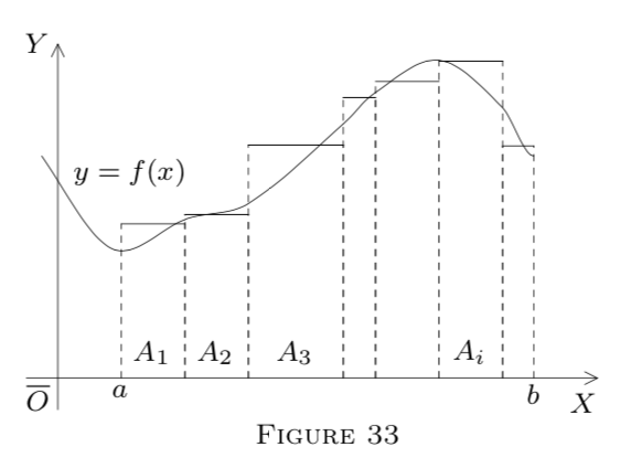
If \(m\) is Lebesgue measure in \(E^{1},\) the integral
\[\int_{A} g=\sum_{i} a_{i} m A_{i}\]
has a simple geometric interpretation; see Figure 33. Let \(A=[a, b] \subset E^{1};\) let \(g\) be bounded and nonnegative on \(E^{1}.\) Each product \(a_{i} m A_{i}\) is the area of a rectangle with base \(A_{i}\) and altitude \(a_{i}.\) (We assume the \(A_{i}\) to be intervals here.) The total area,
\[\int_{A} g=\sum_{i} a_{i} m A_{i},\]
can be treated as an approximation to the area under some curve \(y=f(x)\), where \(f\) is approximated by \(g\) (Theorem 3 in §1). Integration historically arose from such approximations.
Integration of elementary extended-real functions. Note 3 can be extended to sign-changing functions as follows.
If
\[f=\sum_{i} a_{i} C_{A_{i}} \quad\left(a_{i} \in E^{*}\right)\]
on
\[A=\bigcup_{i} A_{i} \quad\left(A_{i} \in \mathcal{M}\right),\]
we set
\[\int_{A} f=\int_{A} f^{+}-\int_{A} f^{-},\]
with
\[f^{+}=f \vee 0 \geq 0 \text { and } f^{-}=(-f) \vee 0 \geq 0;\]
see §2.
By Theorem 2 in §2, \(f^{+}\) and \(f^{-}\) are elementary and nonnegative on \(A;\) so
\[\int_{A} f^{+} \text { and } \int_{A} f^{-}\]
are defined by Note 3, and so is
\[\int_{A} f=\int_{A} f^{+}-\int_{A} f^{-}\]
by our conventions (2*) in Chapter 4, §4.
We shall have use for formula (3), even if
\[\int_{A} f^{+}=\int_{A} f^{-}=\infty;\]
then we say that \(\int_{A} f\) is unorthodox and equate it to \(+\infty,\) by convention; cf. Chapter 4, §4. (Other integrals are called orthodox.) Thus for elementary and (extended) real functions, \(\int_{A} f\) is always defined. (We further develop this idea in §5.)
Note 5. With \(f\) as above, we clearly have
\[f^{+}=a_{i}^{+} \text { and } f^{-}=a_{i}^{-} \text { on } A_{i},\]
where
\[a_{i}^{+}=\max \left(a_{i}, 0\right) \text { and } a_{i}^{-}=\max \left(-a_{i}, 0\right).\]
Thus
\[\int_{A} f^{+}=\sum a_{i}^{+} \cdot m A_{i} \text { and } \int_{A} f^{-}=\sum a_{i}^{-} \cdot m A_{i},\]
so that
\[\int_{A} f=\int_{A} f^{+}-\int_{A} f^{-}=\sum_{i} a_{i}^{+} \cdot m A_{i}-\sum_{i} a_{i}^{-} \cdot m A_{i}.\]
If \(\int_{A} f^{+}<\infty\) or \(\int_{A} f^{-}<\infty,\) we can subtract the two series termwise (Problem 14 of Chapter 4, §13) to obtain
\[\int_{A} f=\sum_{i}\left(a_{i}^{+}-a_{i}^{-}\right) m A_{i}=\sum_{i} a_{i} m A_{i}\]
for \(a_{i}^{+}-a_{i}^{-}=a_{i}.\) Thus formulas (3) and (4) agree with our previous definitions.