7.1: Approximating Definite Integrals as Sums

The standard approach to accumulation is to reduce the problem to an area problem. If we let f(t) be a velocity function, then the area under the y=f(t) curve between a starting value of t=a and a stopping value of t=b is the distance traveled in that time period. In the easiest case, the velocity is constant and we use the simple formula

\[ distance = velocity * time \nonumber \]

Example 7.1.1: Distance with Constant Speed.

Find the distance traveled if I go 60 mph from 12:30 until 3:00.

Solution

This problem is easy to do without any calculus. If we graph the velocity function

we find the area of the rectangle by taking base times height and noting \(60*(3-0.5)=150\text{.}\) Note that we do the same computation if I ask how much I earn over a period of 2.5 years if I make $60K a year, or how much oil is produced in 2 and a half hours form an oil well that produces 60 barrels of oil an hour.

In a similar manner, if the function I am accumulating is linear, I can find area by using the area formula of a triangle, one half base time height.

Example 7.1.2: Approximating Area under a Quadratic Functions.

The question becomes more difficult when I want to find the area under a curve that is not linear. Suppose for example that we want to find the area under the curve

\[ y = x * (4-x) \nonumber \]

between x=0 and x=4.

Solution

We no longer have a nice formula from geometry for the area. Thus we start making approximations. The easiest approximation is to note that the area has to be less than the area of the 4 by 4 rectangle we can draw around the region.

We can improve our estimate by dividing the interval [0, 4] into 4 equal subintervals and then taking the combined area of the 4 rectangles we need to contain the region. This reduces our upper estimate from 16 to 14.

Similarly we could get a better estimate by looking at 8 subintervals and seeing that the area under the parabola is no more than 12.5

If we continue the process with 100 subintervals, our estimate is down to 10.83. From the picture, it looks like a fairly good estimate.

We can change the number of subdivisions with the interactive below.

Figure \(7.1.3.\) GeoGebra: Upper sum approximation

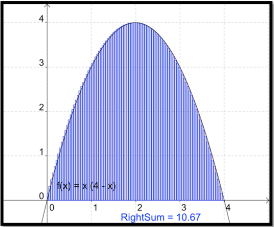
While this process would be very long and tedious by hand, the process of finding the area of each of 100 rectangles and adding the areas is rather easy in Excel. Before going to Excel, we want to make a small adjustment in our method. The method we used always gives an overestimate. It also requires that we know where the function reaches a maximum on each subinterval. It will be easier if we estimate area by always taking the height of the rectangle at the right end of the subinterval. With 4 subintervals this gives an estimate of 10 for our area.

When we increase the number of subintervals to 100, we once again get a fairly good estimate of the area. From the picture, it is hard to see difference between the area defined by the curve and the area defined by the rectangles.

Example 7.1.4:

Find the area under the curve \(y=x*(4-x)\) with \(x\) between 0 and 4 with Excel

Solution

We will approximate the area with 100 rectangles. We set up a worksheet to find the area of the first rectangle.

Following our standard practice, we set up the question and answer in labeled areas at the top of the worksheet. The width of a subinterval is the width of the whole interval divided by the number of subintervals. The column \(x_n\) is for the x value at the right side of the n-th subinterval. The value of \(x_n\) is the starting point plus n times the width of a subinterval. We then evaluate the function at \(x_n\text{.}\) The area of the n-th rectangle is the height, or \(f(x_n)\text{,}\) times the width of the subinterval. The last column is the total area for the first n rectangles. The area for 100 rectangles is our area estimate.

To find the area we quick fill our worksheet.

For a more accurate estimate we divide into smaller rectangles.

While 100 subintervals will be close enough for most of the problems we are interested is, the "area", or definite integral will be defined as the limit of this sum as the number of subintervals goes to infinity. Thus

\[ \int_a^bf(x) dx=\lim_{n\to \infty} \sum_{i=1}^nf (x_i)\Delta x \nonumber \]

with \(\Delta x=\frac{b-a}{n}\) and \(x_i=a+i*\Delta x\text{.}\)

The sums of the form, \(\sum_{i=1}^n f(x_i)\Delta x\) with \(\Delta x=\frac{b-a}{n}\) and \(x_i=a+i*\Delta x\text{,}\) are called Riemann sums. The limit, written \(\int_a^bf(x) dx\text{,}\) is called a definite integral.

As a memory aid, it is worth noting that the symbol used for the sum is an upper case sigma, or S for sum in the Greek alphabet. When we take the limit we use an integral sign, which is a stylized S in the Latin alphabet.

It is worth noting that in this definition we are finding “signed area under a curve.” If the function \(f(x)\) is negative over the interval, the integral will also be negative, in the same we would have a negative change in our bank statement if we were steadily removing money. Similarly we can get a negative integral when the ends of the interval are reversed. If I am steadily adding money to an account, the net change is negative if I measure from 5 years in the future back to today.

We should note that, for functions nice enough to be considered in this class, we get to the same limit by using rectangles with the function evaluated on the right side of the rectangle or the left side of the rectangle, or any point in the rectangle we choose. Choosing the right hand side for evaluation makes our formulas a little simpler.

Example 7.1.5: Present Value of a Revenue Stream.

The estimated current value of the revenue stream, in billions of dollars, of a company being bought out is \(f(x)=\exp(-0.06*x)*0.235\text{.}\) The present value of that revenue stream is the area of the region under the curve \(y=f(x)\) from \(x=0\) to \(x=15\text{.}\) Use 500 intervals to estimate the present value.

Solution

Although the data in the question for this example is quite different from the previous example, the setup for the worksheet to evaluate the Riemann sum is the same.

With 500 intervals we estimate the present value of the revenue stream to be worth $2.3222 Billion. If we had only used 100 intervals, the estimate would have been for $2.318 Billion, while 1000 intervals gives an estimate of $2.3232 Billion.

Exercises: Approximating Definite Integrals as Sums Problems

Exercise 1:

Let \(f(x) = 4 x + 5\text{.}\) Estimate the area under \(f(x)\) on the interval \(0 \le x \lt 7\) using 100 rectangles and a right hand rule.

Answer

The Excel commands are:

The answer is given as follows. Note that in this screen grab the center part of the sidebyside was hidden so that the image is a reasonable size

The area is approximately 133.98