
10.5: Application - Inflation, Purchasing Power, and Rates Of Change
- Page ID
- 22128

How much does inflation cut into people’s incomes and wealth? In 1955, the average Canadian worker earned an annual gross salary of about $2,963.1 By 2010, the average Canadian worker brought home annual gross earnings approximating $44,366.2 Does this mean that Canadians today are 15 times richer than our grandparents? From earlier discussions in section 4.3 on inflation, real income, and purchasing power, you already can tell we are not. The actual increase is by something less than 15 times. But how much less is it?
To answer the question, you have to express both incomes with reference to the same year. Either convert the 1955 income to its 2010 equivalent or vice versa. To help, what if you are told the rate of inflation from 1955 to 2010 averaged 3.91%3 per year? To convert, you might use either the percent change method or the real income method. Each of these poses problems, though:
• To use the percent change formula from section 3.1, you would have to apply it 55 consecutive times! Clearly, this is impractical.
• To use the real income formula from section 4.3, you would need the consumer price index numbers for both years. Locating CPI values can be time consuming, especially for years in the distant past. Another complication is that if you want to project future values (such as the equivalent income in, say, 2020 instead of 2010), CPI values do not exist for future years.
There has to be an easier way! In this section, you will see how to adapt the compound interest concepts and formulas to suit such applications as inflation, purchasing power, and even percent change.
Inflation
Inflation is the overall upward price movement of products in an economy. It is measured by positive change in the consumer price index. Historical inflation rates in Canada are illustrated in the figure below.
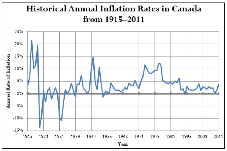
Note that historically prices have always risen over the long term. In the short term, though, there have been periods during which prices moved downward. This is known as deflation, which is measured by negative change in the consumer price index. Such periods of deflation usually do not last very long; the longest period recorded was during the Great Depression. Most recently, deflation occurred for a few months in 2009.
Inflation is most commonly expressed as an annual rate; therefore, you treat it mathematically as an annually compounded interest rate. This is the nominal interest rate (\(IY\)) with a compounding frequency of one, or \(CY\) = 1. Note that if deflation has occurred during the time period in question, the interest rate is a negative number. If you have a series of inflation rates, you treat this as a variable interest rate. If you are finding an average inflation rate for some time period, you treat this like finding the equivalent fixed interest rate. In using the compound interest formulas, assign the present value to any beginning value in the problem at hand, while the future value is any ending value. The number of compounding periods (\(N\)) still reflects the number of compounds between the two values.
How It Works
You can use any of the formulas and techniques from Chapter 9 to work with inflation. The opening example of incomes in 1955 and 2010 will illustrate the processes.
Solving for Future Value
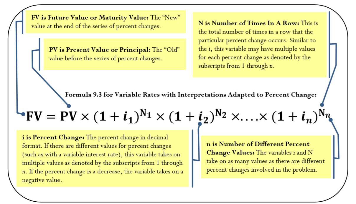
If the unknown variable is an ending value, apply Formula 9.3, solving for the future value. If only one inflation rate (a fixed rate) applies, this requires only one application of the formula. If the inflation rate changes over time, you apply the formula multiple times or use the quick method of calculation:
\[FV=PV \times\left(1+i_{1}\right)^{N_{1}} \times\left(1+i_{2}\right)^{N_{2}} \times \ldots \times\left(1+i_{n}\right)^{N_{n}} \nonumber \]
In the example, you could move the 1955 income to 2010. In this case, the \(PV\) = $2,963, \(IY\) = 3.91%, \(CY\) = 1, and \(N\) = 55. With a fixed interest rate, apply Formula 9.3 and calculate \(FV = $2,963(1 + 0.0391)^{55} = $24,427.87\). Therefore, the 2010 equivalent income of 1955 is approximately $24,427. Note the actual 2010 income is about 81% higher, which would imply that Canadians have indeed become wealthier.
Solving for Present Value
If the unknown variable is a beginning value, apply Formula 9.3, rearranging for present value. Depending on whether the inflation rate is fixed or variable, solve using the same technique as for future value. In the example, you could move the 2010 income to 1955. In this case, the \(FV\) = $44,366, \(IY\) = 3.91%, \(CY\) = 1, and \(N\) = 55. With a fixed interest rate, apply Formula 9.3, rearranging for \(PV\), and calculate \(PV\) = $44,366 ÷ (1 + 0.0391)55 = $5,381.41. Therefore, the 1955 equivalent income of 2010 is approximately $5,381. Note this income is the same percentage (81%) higher than the actual 1955 income, as you found by the first method.
Solving for the Rate
If the average inflation rate is the unknown variable, then the beginning and ending values must be known. In the example, assume the average inflation rate is unknown, but the equivalent incomes of \(PV\) =$2,963 in 1955 and \(FV\) = $24,427.87 in 2010 are known. The \(CY\) = 1 and \(N\) = 55 years. Applying Formula 9.3 results in \(\$24,427.87 = \$2,963(1 + i)^{55}\). Solving for \(i\) you get 3.91%. This is the average inflation rate (since \(CY\) = 1, then \(i = IY\)).
Solving for the Term
If the unknown variable is the amount of time between the beginning and ending values, once again apply Formula 9.3 and rearrange for \(N\). In the example, assume the beginning and ending values of \(PV\) = $2,963 in 1955 and \(FV\) = $24,427.87 are known, but the year for the future value is unknown. The \(IY\) = 3.91% and \(CY\) = 1. Applying Formula 9.3 gives you \(\$24,427.87 = $2,963(1 + 0.0391)^N\). Solving for \(N\) gives 55 years. The starting year of 1955 + 55 years is the ending year of 2010, in which the equivalent income of $24,427.87 applies.
Important Notes
Your BAII Plus Calculator
The time value of money buttons are designed for financial calculations and require you to follow the cash flow sign convention at all times. Remember that this convention requires money leaving you to be entered as a negative number, and money being received by you to be entered as a positive number.
When you adapt this function to economic calculations such as inflation, no money is being invested or received— numbers are being moved across time. To obey the calculator requirement of the cash flow sign convention, ensure that the signs attached to the present (\(PV\)) and future values (\(FV\)) are opposites. The choice as to which is positive and which is negative is arbitrary and does not affect the outcome of the calculation. Ignore the cash flow sign displayed on any solutions.
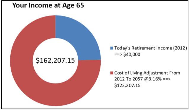
Many experts today claim that the average Canadian retiree in 2012 needs approximately $40,000 in gross annual income to retire comfortably. Assume that you are 20 years old in 2012. Historically in Canada, the inflation rate has averaged 3.16%. If the average inflation rate continues in the future, what gross income will you require when you retire at age 65?
Solution
Calculate the ending value (\(FV\)) for your annual gross income when you retire at age 65.
What You Already Know
Step 1:
The present value, fixed inflation rate, and time frame are known, as illustrated in the timeline.
Years = 45

How You Will Get There
Step 2:
With a \(CY\) = 1, the \(i = IY\).
Step 3:
Apply Formula 9.2 to calculate the number of compounding periods.
Step 4:
Calculate the future value by applying Formula 9.3.
Perform
Step 2:
\(i\) = 3.16%
Step 3:
\(N\) = 1 × 45 = 45
Step 4:
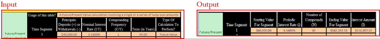
\(FV = \$40,000(1 + 0.0316)^{45} = \$162,207.15\)
| N | I/Y | PV | PMT | FV | P/Y | C/Y |
|---|---|---|---|---|---|---|
| 45 | 3.16 | -40000 | 0 | Answer: 160,798.0247 | 1 | 1 |
When you retire in 2057, if inflation continues to average 3.16% annually, according to the experts your annual gross income must be $162,207.15 for you to live comfortably.
Excel Instructions
Open the Excel template entitled “Chapter 9: Single Payments and Compound Interest Template.”
Purchasing Power
Recall from section 4.3 that the purchasing power of a dollar is the amount of goods and services that can be exchanged for a dollar. Purchasing power has an inverse relationship to inflation. When inflation occurs and prices increase, your purchasing power decreases.
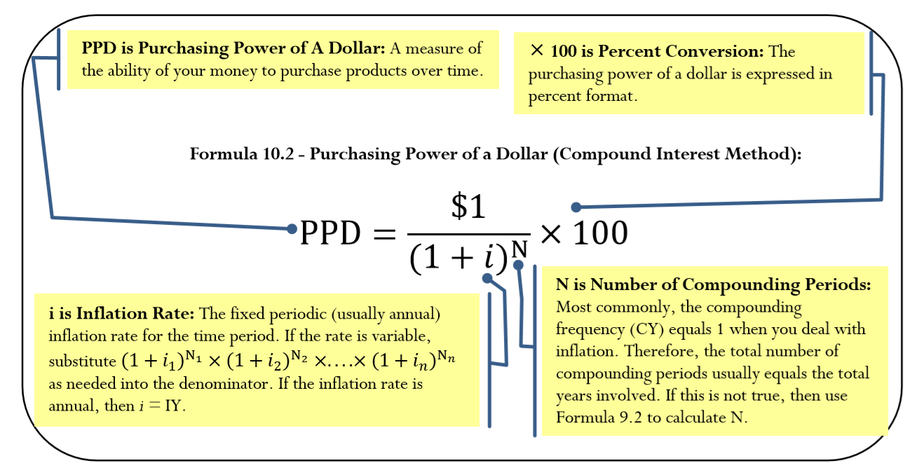
The Formula
In the formula introduced in section 4.3, the denominator used the CPI to represent the change in product prices. In compound interest applications, you instead use the inflation rate, as shown in Formula 10.2.
How It Works
Follow these steps to solve a purchasing power question using compound interest:
Step 1: Identify the inflation rate (\(IY\)), the compounding on the inflation rate (\(CY\)), and the term (Years). Normally, \(i = IY\) and \(N\) = Years; however, apply Formula 9.1 and Formula 9.2 if you need to calculate \(i\) or \(N\).
Step 2: Apply Formula 10.2, solving for the purchasing power of a dollar.
Using the income example, determine how an individual's purchasing power has changed from 1955 to 2010. Recall that the average inflation during the period was 3.91% per year.
Step 1: The \(IY\) = 3.91%, \(CY\) = 1, and Years = 55. The annual rate lets \(i\) = 3.91% and \(N\) = 54.
Step 2: From Formula 10.2, the \(PPD=\dfrac{\$ 1}{(1+0.0391)^{55}} \times 100=12.1296 \%\). As a rough interpretation, this means that if someone could purchase 100 items with $100 in 1955, that same $100 would only purchase about 12 of the same items in 2010.
Things To Watch Out For
Determine exactly what the question is asking you to calculate with respect to the purchasing power of a dollar.
- If the question asks, "What is the purchasing power of a dollar?" then your answer is the result of Formula 10.2.
- If the questions asks, "How has your purchasing power decreased?" then your answer is 100% minus the result of Formula 10.2.
It is critical to Plan when solving these questions so that your solution addresses the question asked.
What is the purchasing power of your dollar if the prices on products:
- Double?
- Triple?
- Quadruple?
- Answer
-
- 1/2 = 50%
- 1/3 = \(3.3\bar{3}\%\)
- 1/4 = 25%
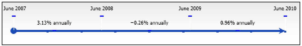
The historical inflation rates in Canada were 3.13% from June 2007 to June 2008, −0.26% from June 2008 to June 2009, and 0.96% from June 2009 to June 2010. Comparing June 2007 to June 2010, what is the purchasing power of a 2007 dollar in 2010?
Solution
Calculate the purchasing power of a 2007 dollar (\(PPD\)) in 2010.
What You Already Know
Step 1:
The inflation rates and terms are known, as illustrated in the timeline.
\(CY\) (for each time segment) = 1, Term (for each time segment) = 1 Year
How You Will Get There
Step 1 (continued):
Identify the periodic interest rate (\(i\)) and the number of compounds (\(N\)) for each time segment. With \(CY\) = 1, then \(i = IY\) and \(N\) = Years.
Step 2:
Apply Formula 10.2, substituting the variable interest rate version in the denominator.
Perform
Step 1 (continued):
\(i_1\) = 3.13%, \(i_2\) = −0.26%, \(i_3\) = 0.96%; \(N_1, N_2, N_3\) = 1
Step 2:
\[\begin{aligned}
PPD &=\dfrac{\$ 1}{(1+0.0313) \times(1-0.0026) \times(1+0.0096)} \times 100 \\
&=96.2933 \%
\end{aligned} \nonumber \]
Calculator Instructions
| Time Segment | N | I/Y | PV | PMT | FV | P/Y | C/Y |
|---|---|---|---|---|---|---|---|
| 1 | 1 | 3.13 | Answer: 0.969649 | 0 | -1 | 1 | 1 |
| 2 | \(\surd\) | -0.26 | Answer: 0.972177 | \(\surd\) | -0.969649 | \(\surd\) | \(\surd\) |
| 3 | \(\surd\) | 0.96 | Answer: 0.962933 | \(\surd\) | -0.972177 | \(\surd\) | \(\surd\) |
The purchasing power of a June 2007 dollar in June 2010 is 96.2933%. If $100 in June 2007 could purchase 100 items, in June 2010 $100 could only purchase about 96 items.
Rates of Change
Recall from section 3.1 that you could calculate a percent change between Old and New numbers. While this formula works well when you are interested in just a single percent change, it becomes time consuming and tedious when you work with a series of percent changes. For example, assume the \(TSX\) has a value of 12,000. The \(TSX\) then drops by 4% each month for five months, and then rises by 4% each month for five months. What is the “New” value for the \(TSX\)? It is not 12,000! If you use the formula for percent change, you need a series of 10 calculations solving for “New” each time—one calculation for each month! Not much fun. Mathematically, in a series of percent changes, each change compounds on the previous one. Therefore, you can use compound interest formulas to work with any series of percent changes.
The Formula
You can solve any series of percent changes by applying an adapted version of Formula 9.3 for variable interest rates:
How It Works
Follow these steps to adapt Formula 9.3 for percent change applications:
Step 1: Assign either the “Old” value to \(PV\) or the “New” value to \(FV\) (depending on which you know).
Step 2: Identify your series of percent changes (\(i_1\) through \(i_n\)) and how many times in a row each percent change value occurs (\(N_1\) through \(N_n\)). Remember that decreases are negative values.
Step 3: Apply the adapted version of Formula 9.3, solving for either \(FV\) or \(PV\).
As an example, find out the new value for the \(TSX\) based on a starting value of 12,000 with decreases of 4% for five months followed by increases of 4% for five months.
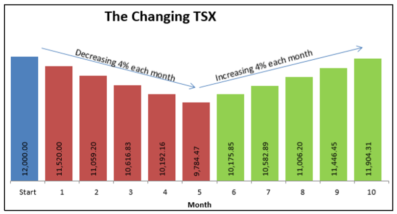
Step 1: The “Old” value is \(PV\)=12,000.
Step 2: The first change is a decrease of 4%, or \(i_1\) = −4%. It occurs for five months in a row, thus \(N_1\) = 5. Next, an increase of 4%, or \(i_2\) = 4%, also occurs five months in a row, thus \(N_2\) = 5.
Step 3: Use Formula 9.3 to calculate \(FV = 12,000 × (1 − 0.04)^5 × (1 + 0.04)^5 = 11,904.31\). The “New” value of the \(TSX\) after the 10 months of change is 11,904.31.
Important Notes
You can use your financial calculator for these nonfinancial calculations just as you did for inflation. You must follow the cash flow sign convention by ensuring that \(PV\) and \(FV\) have opposite signs. However, once again the signs do not have any meaning in these calculations.
Things To Watch Out For
When you work with variable inflation rates, purchasing power of a dollar, or rates of change, you can simplify the variable rates into a single fixed rate using a geometric average before applying the compound interest formula. For example, using the \(TSX\) example above, the geometric average of the 10 months of change is:
\[GAvg =\left [\sqrt[10]{(1-0.04)^{5} \times(1+0.04)^{5}}-1 \right] \times 100=-0.080032 \% \nonumber \]
Using this calculated value as the periodic interest rate and substituting into Formula 9.3 produces:
\[FV = 12,000 × (1 − 0.00080032)^{10} = 11,904.31\nonumber \]
Similarly, you could solve Example \(\PageIndex{2}\) with this approach. Some students have found this technique easier than working with the variable rates. Either way, whether you use variable rates or the geometric average as the fixed rate, both techniques produce the same solution.
If a quantity decreases by \(x\%\) and then increases by the same percent, why do you not arrive at the original quantity as your “New” value?
- Answer
-
The initial decrease will make the base number smaller. If the new base number is then increased by the same percentage, that percentage is determined from a smaller base. It will not produce the same value as the decrease.
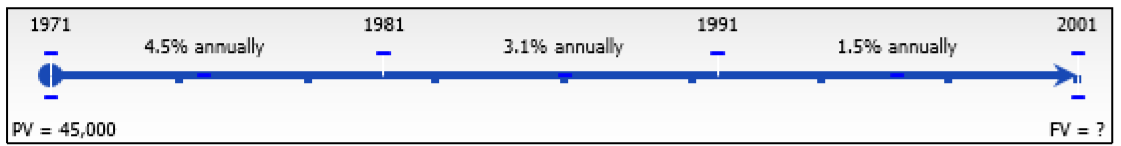
The City of Vancouver tracks employment in its Metro Core area. In 1971, approximately 45,000 employees in the Metro Core area were classified as "professional and commercial service" workers. From 1971 to 1981, the number of workers grew by about 4.5% per year. From 1981 to 1991, the growth rate was about 3.1% per year, and from 1991 to 2001 the growth rate was about 1.5% per year.4 Rounded to the nearest thousand, how many people were employed in the "professional and commercial services" field in the Metro Core area of Vancouver in 2001?
Solution
You are looking for the “New” value (\(FV\)) of the number of employees after the 30 years of percent changes.
What You Already Know
Step 1:
The beginning value and structure of the sequence of percent changes are known, as shown in the timeline.
How You Will Get There
Step 2:
Capture the values of \(i_n\) and \(N_n\) for each consecutive percent change value. Note that the timeline has three time segments, so each variable has three values.
Step 3:
Apply Formula 9.3.
Perform
Step 2:
\[i_{1}=4.5 \%, N_{1}=10, i_{2}=3.1 \%, N_{2}=10, i_{3}=1.5 \%, N_{3}=10 \nonumber \]
Step 3:
\[\begin{aligned}
&FV=45,000 \times(1+0.045)^{10} \times(1+0.031)^{10} \times(1+0.015)^{10}\\
&FV=45,000 \times 1.045^{10} \times 1.031^{10} \times 1.015^{10}\\
&FV=45,000 \times 1.552969 \times 1.357021 \times 1.160540=110,058=110,000
\end{aligned} \nonumber \]
Calculator Instructions
| Time Segment | N | I/Y | PV | PMT | FV | P/Y | C/Y |
|---|---|---|---|---|---|---|---|
| 1 | 10 | 4.5 | -45000 | 0 | Answer: 69,883.62398 | 1 | 1 |
| 2 | \(\surd\) | 3.1 | -69,883.62398 | \(\surd\) | Answer: 94,833.56372 | \(\surd\) | \(\surd\) |
| 3 | \(\surd\) | 1.5 | -94,833.56372 | \(\surd\) | Answer: 110,058.2223 | \(\surd\) | \(\surd\) |
From 1971 to 2001, the number of employees in the "professional and commercial services" field in the Metro Core area of Vancouver grew from 45,000 to 110,000.
References
- Statistics Canada, “Average Annual, Weekly and Hourly Earnings, Male and Female Wage-Earners, Manufacturing Industries, Canada, 1934 to 1969,” adapted from Series E60–68, www.statcan.gc.ca/pub/11-516-x/sectione/E60_68eng.csv, accessed July 28, 2010.
- Statistics Canada, “Earnings, Average Weekly, by Province and Territory,” adapted from CANSIM table 281-0027 and Catalogue no. 72-002-X, www40.statcan.gc.ca/l01/cst01/labr79-eng.htm, accessed August 11, 2011.
- Statistics Canada, “Consumer Price Indexes for Canada, Monthly, 1914–2012 (V41690973 Series)”; all values based in May of each year; www.bankofcanada.ca/rates/related/inflation-calculator/?page_moved=1, accessed November 26, 2012.
- City of Vancouver, “Employment Change in the Metro Core,” November 22, 2005, http://s3.amazonaws.com/zanran_stora...es/7116122.pdf, accessed August 20, 2013