11.3: Present Value Of Annuities
- Page ID
- 22133

\( \newcommand{\vecs}[1]{\overset { \scriptstyle \rightharpoonup} {\mathbf{#1}} } \)
\( \newcommand{\vecd}[1]{\overset{-\!-\!\rightharpoonup}{\vphantom{a}\smash {#1}}} \)
\( \newcommand{\dsum}{\displaystyle\sum\limits} \)
\( \newcommand{\dint}{\displaystyle\int\limits} \)
\( \newcommand{\dlim}{\displaystyle\lim\limits} \)
\( \newcommand{\id}{\mathrm{id}}\) \( \newcommand{\Span}{\mathrm{span}}\)
( \newcommand{\kernel}{\mathrm{null}\,}\) \( \newcommand{\range}{\mathrm{range}\,}\)
\( \newcommand{\RealPart}{\mathrm{Re}}\) \( \newcommand{\ImaginaryPart}{\mathrm{Im}}\)
\( \newcommand{\Argument}{\mathrm{Arg}}\) \( \newcommand{\norm}[1]{\| #1 \|}\)
\( \newcommand{\inner}[2]{\langle #1, #2 \rangle}\)
\( \newcommand{\Span}{\mathrm{span}}\)
\( \newcommand{\id}{\mathrm{id}}\)
\( \newcommand{\Span}{\mathrm{span}}\)
\( \newcommand{\kernel}{\mathrm{null}\,}\)
\( \newcommand{\range}{\mathrm{range}\,}\)
\( \newcommand{\RealPart}{\mathrm{Re}}\)
\( \newcommand{\ImaginaryPart}{\mathrm{Im}}\)
\( \newcommand{\Argument}{\mathrm{Arg}}\)
\( \newcommand{\norm}[1]{\| #1 \|}\)
\( \newcommand{\inner}[2]{\langle #1, #2 \rangle}\)
\( \newcommand{\Span}{\mathrm{span}}\) \( \newcommand{\AA}{\unicode[.8,0]{x212B}}\)
\( \newcommand{\vectorA}[1]{\vec{#1}} % arrow\)
\( \newcommand{\vectorAt}[1]{\vec{\text{#1}}} % arrow\)
\( \newcommand{\vectorB}[1]{\overset { \scriptstyle \rightharpoonup} {\mathbf{#1}} } \)
\( \newcommand{\vectorC}[1]{\textbf{#1}} \)
\( \newcommand{\vectorD}[1]{\overrightarrow{#1}} \)
\( \newcommand{\vectorDt}[1]{\overrightarrow{\text{#1}}} \)
\( \newcommand{\vectE}[1]{\overset{-\!-\!\rightharpoonup}{\vphantom{a}\smash{\mathbf {#1}}}} \)
\( \newcommand{\vecs}[1]{\overset { \scriptstyle \rightharpoonup} {\mathbf{#1}} } \)
\(\newcommand{\longvect}{\overrightarrow}\)
\( \newcommand{\vecd}[1]{\overset{-\!-\!\rightharpoonup}{\vphantom{a}\smash {#1}}} \)
\(\newcommand{\avec}{\mathbf a}\) \(\newcommand{\bvec}{\mathbf b}\) \(\newcommand{\cvec}{\mathbf c}\) \(\newcommand{\dvec}{\mathbf d}\) \(\newcommand{\dtil}{\widetilde{\mathbf d}}\) \(\newcommand{\evec}{\mathbf e}\) \(\newcommand{\fvec}{\mathbf f}\) \(\newcommand{\nvec}{\mathbf n}\) \(\newcommand{\pvec}{\mathbf p}\) \(\newcommand{\qvec}{\mathbf q}\) \(\newcommand{\svec}{\mathbf s}\) \(\newcommand{\tvec}{\mathbf t}\) \(\newcommand{\uvec}{\mathbf u}\) \(\newcommand{\vvec}{\mathbf v}\) \(\newcommand{\wvec}{\mathbf w}\) \(\newcommand{\xvec}{\mathbf x}\) \(\newcommand{\yvec}{\mathbf y}\) \(\newcommand{\zvec}{\mathbf z}\) \(\newcommand{\rvec}{\mathbf r}\) \(\newcommand{\mvec}{\mathbf m}\) \(\newcommand{\zerovec}{\mathbf 0}\) \(\newcommand{\onevec}{\mathbf 1}\) \(\newcommand{\real}{\mathbb R}\) \(\newcommand{\twovec}[2]{\left[\begin{array}{r}#1 \\ #2 \end{array}\right]}\) \(\newcommand{\ctwovec}[2]{\left[\begin{array}{c}#1 \\ #2 \end{array}\right]}\) \(\newcommand{\threevec}[3]{\left[\begin{array}{r}#1 \\ #2 \\ #3 \end{array}\right]}\) \(\newcommand{\cthreevec}[3]{\left[\begin{array}{c}#1 \\ #2 \\ #3 \end{array}\right]}\) \(\newcommand{\fourvec}[4]{\left[\begin{array}{r}#1 \\ #2 \\ #3 \\ #4 \end{array}\right]}\) \(\newcommand{\cfourvec}[4]{\left[\begin{array}{c}#1 \\ #2 \\ #3 \\ #4 \end{array}\right]}\) \(\newcommand{\fivevec}[5]{\left[\begin{array}{r}#1 \\ #2 \\ #3 \\ #4 \\ #5 \\ \end{array}\right]}\) \(\newcommand{\cfivevec}[5]{\left[\begin{array}{c}#1 \\ #2 \\ #3 \\ #4 \\ #5 \\ \end{array}\right]}\) \(\newcommand{\mattwo}[4]{\left[\begin{array}{rr}#1 \amp #2 \\ #3 \amp #4 \\ \end{array}\right]}\) \(\newcommand{\laspan}[1]{\text{Span}\{#1\}}\) \(\newcommand{\bcal}{\cal B}\) \(\newcommand{\ccal}{\cal C}\) \(\newcommand{\scal}{\cal S}\) \(\newcommand{\wcal}{\cal W}\) \(\newcommand{\ecal}{\cal E}\) \(\newcommand{\coords}[2]{\left\{#1\right\}_{#2}}\) \(\newcommand{\gray}[1]{\color{gray}{#1}}\) \(\newcommand{\lgray}[1]{\color{lightgray}{#1}}\) \(\newcommand{\rank}{\operatorname{rank}}\) \(\newcommand{\row}{\text{Row}}\) \(\newcommand{\col}{\text{Col}}\) \(\renewcommand{\row}{\text{Row}}\) \(\newcommand{\nul}{\text{Nul}}\) \(\newcommand{\var}{\text{Var}}\) \(\newcommand{\corr}{\text{corr}}\) \(\newcommand{\len}[1]{\left|#1\right|}\) \(\newcommand{\bbar}{\overline{\bvec}}\) \(\newcommand{\bhat}{\widehat{\bvec}}\) \(\newcommand{\bperp}{\bvec^\perp}\) \(\newcommand{\xhat}{\widehat{\xvec}}\) \(\newcommand{\vhat}{\widehat{\vvec}}\) \(\newcommand{\uhat}{\widehat{\uvec}}\) \(\newcommand{\what}{\widehat{\wvec}}\) \(\newcommand{\Sighat}{\widehat{\Sigma}}\) \(\newcommand{\lt}{<}\) \(\newcommand{\gt}{>}\) \(\newcommand{\amp}{&}\) \(\definecolor{fillinmathshade}{gray}{0.9}\)Have you ever noticed that the prices of expensive products are generally not advertised? Instead, companies that market these high-ticket products promote the payment amounts of the annuity, not the actual sticker price. In fact, locating the actual price for these products in the advertisements usually requires a magnifying glass. For example, a Mitsubishi Outlander was recently advertised for only $193 biweekly. That does not sound so bad, and perhaps you might be tempted to head on down to the car dealership to buy one of those vehicles. However, the fine print indicates that you need to make 182 payments, which then total almost $32,000. Why is the vehicle advertised this way? Numerically, $193 sounds a lot better than $32,000!
In business, whether you are setting up consumers with payment plans or buying and selling loan contracts, you need to calculate present values. As a consumer, you encounter present value calculations in many ways:
- How to take advertised payment amounts and convert them to the actual price that you must pay.
- Meeting financial goals by planning your RRSP, which requires knowing how much money you need at the start.
This section develops present value formulas for both ordinary annuities and annuities due. Like future value calculations, these formulas accommodate both simple and general annuities as needed. From investments, we will then extend annuity calculations to loans as well.
Ordinary Annuities and Annuities Due
The present value of any annuity is equal to the sum of all of the present values of all of the annuity payments when they are moved to the beginning of the first payment interval. For example, assume you will receive $1,000 annual payments at the end of every payment interval for the next three years from an investment earning 10% compounded annually. How much money needs to be in the annuity at the start to make this happen? In this case, you have an ordinary simple annuity. The figure below illustrates the fundamental concept of the time value of money and shows the calculations in moving all of the payments to the focal date at the start of the timeline.
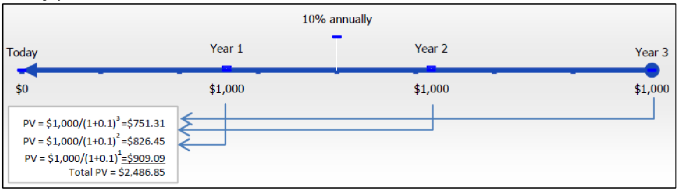
Observe that all three payments are present valued to your focal date, requiring an investment of $2,486.85 today. In contrast, what happens to your timeline and calculations if those payments are made at the beginning of every payment interval? In this case, you have a simple annuity due. The next figure illustrates your timeline and calculations.
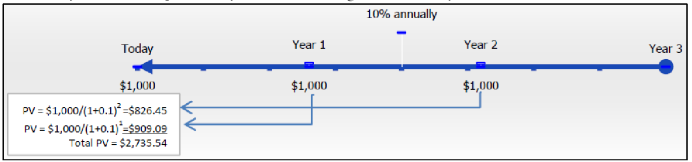
Observe that only two of the three payments need to be present valued to your focal date since the first payment is already on the focal date. The total investment for an annuity due is higher at $2,735.54 because the first payment is withdrawn immediately, so a smaller principal earns less interest than does the ordinary annuity.
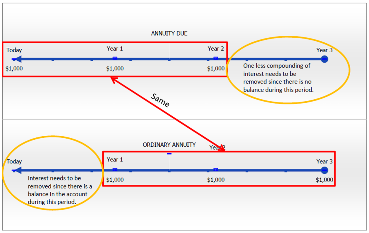
The next figure below contrasts the two annuity types. Working from right to left on the timeline, the key difference is that the annuity due has one less compound of interest to remove. Its first time segment (from the right) contains a zero balance, while the ordinary annuity does contain a balance that needs to have interest discounted. Note that if you take the annuity due and remove one extra compound of interest, you arrive at $2,735.54 ÷ (1 + 0.1) = $2,486.85, which is the present value of the corresponding ordinary annuity.
The Formula
As with future value calculations, calculating present values by manually moving each payment to its present value is extremely time consuming when there are more than a few payments. Similarly, annuity formulas allow you to move all payments simultaneously in a single calculation. The formulas for ordinary annuities and annuities due are presented together.
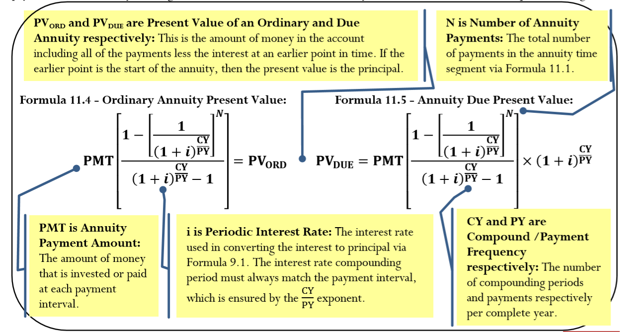
The following observations are made about these two formulas:
- The formulas adapt to both simple and general annuities. In the case of simple annuities, the compounding frequency already matches the payment frequency, so it requires no conversion; numerically, the exponent of \(\dfrac{CY}{PY}\) produces a quotient of 1 and removes itself from the formula. In the case of general annuities, the exponent converts the compounding frequency of the interest rate to match the payment frequency.
- Identical in structure to the future value formulas, these two formulas for present value are also complex equations involving rate, portion, and base. Here the present value (\(PV_{ORD}\) or \(PV_{DUE}\)) = portion, \(PMT\) = base, and everything else = rate. The numerator, \(1-\left[\dfrac{1}{(1+i)^{\frac{CY}{PY}}}\right]^{N}\), produces the overall percent decrease in the annuity; the denominator, \((1+i)^{\frac{CY}{PY}}-1\), produces the percent change with each payment; the division of these two percent changes creates a ratio by which present value relates to the annuity payment itself. To illustrate, assume that \(i\) = 5%, \(N\) = 2, and \(CY = PY\) = 1. Substituting these numbers into the formula gives the following: \[\dfrac{1-\left[\dfrac{1}{(1+i)^{\frac{CY}{PY}}}\right]^N}{(1+i)^{\frac{CY}{PY}}-1}=\dfrac{1-\left[\dfrac{1}{(1+.05)^{\frac{1}{1}}}\right]^{2}}{(1+.05)^{\frac{1}{1}}-1}=\dfrac{0.092970}{0.05}=1.859410 \nonumber \]From these numbers, it is evident that the present value amount represents a decrease of 9.2970% (the numerator) overall. With each payment, the decrease is 5% (the denominator). Therefore, the ratio of the present value overall to each payment (the \(PMT\)) is 1.859410. If the annuity payment amount is \(PMT\) = $1,000, then the value of the \(PV_{ORD}=\$ 1,000(1.859410)=\$ 1,859.41\).
- The only difference from an ordinary annuity is the multiplication of the extra term \((1+i)^{\frac{CY}{PY}}\). The multiplication results in the removal of one fewer compounds of interest than the ordinary annuity.
How It Works
Follow these steps to calculate the present value of any ordinary annuity or annuity due:
Step 1: Identify the annuity type. Draw a timeline to visualize the question.
Step 2: Identify the variables that you know, including \(FV, IY, CY, PMT, PY\), and Years.
Step 3: Use Formula 9.1 to calculate \(i\).
Step 4: If \(FV\) = $0, proceed to step 5. If there is a nonzero value for \(FV\), treat it like a single payment. Apply Formula 9.2 to determine \(N\) since this is not an annuity calculation. Move the future value to the beginning of the time segment using Formula 9.3, rearranging for \(PV\).
Step 5: Use Formula 11.1 to calculate \(N\). Apply either Formula 11.4 or Formula 11.5 based on the annuity type. If you calculated a present value in step 4, combine the present values from steps 4 and 5 to arrive at the total present value.
Important Notes
Calculating the Interest Amount. If you are interested in knowing how much interest was removed in the calculation of the present value, adapt Formula 8.3, where \(I = S – P = FV − PV\). The present value (\(PV\)) is the solution to either Formula 11.4 or Formula 11.5. The \(FV\) in Formula 8.3 is expanded to include the sum of all future monies, so it is replaced by \(N × PMT + FV\). Therefore, you rewrite Formula 8.3 as \(I = (N × PMT + FV) − PV\).
Your BAII+ Calculator. If a single payment future value (FV) is involved in a present value calculation, then you require two formula calculations using Formula 9.3 and either Formula 11.4 or Formula 11.5. The calculator performs both of these calculations simultaneously if you input values obeying the cash flow sign convention for both \(FV\) and \(PMT\).
For two equal investment annuities, will the present value of an ordinary annuity and annuity due be the same or different?
- Answer
-
They will be different. The annuity due always has the larger present value since it removes one fewer compound of interest than the ordinary annuity.
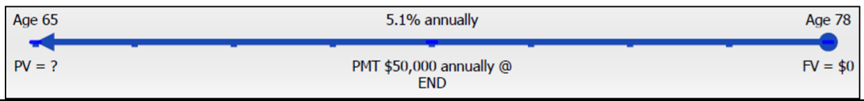
Rodriguez is planning on having an annual gross income of $50,000 at the end of every year when he retires at age 65. He is planning for the account to be emptied by age 78, which is the average life expectancy for a Canadian man. If the account earns 5.1% compounded annually, what amount of funds needs to be in the account when he retires?
Solution
Step 1:
The payments are at the end of the payment intervals, and the compounding period and payment intervals are the same. This is, therefore, an ordinary simple annuity. Calculate its value at the start, which is its present value, or \(PV_{ORD}\).
What You Already Know
Step 1 (continued):
The timeline for the client's account appears below.
Step 2:
\(FV\) = $0, \(IY\) = 5.1%, \(CY\) = 1, \(PMT\) = $50,000, \(PY\) = 1, Years = 13
How You Will Get There
Step 3:
Apply Formula 9.1.
Step 4:
Since \(FV\) = $0, skip this step.
Step 5:
Apply Formula 11.4 and Formula 11.5.
Perform
Step 3:
\(i=5.1 \% \div 1=5.1 \%\)
Step 5:
\(N=1 \times 13=13\) payments
\[PV_{ORD}=\$ 50,000\left[\dfrac{1-\left[\frac{1}{(1+0.051)^{\frac{1}{1}}}\right]^{13}}{(1+0.051)^{\frac{1}{1}}-1}\right]=\$ 466,863.69 \nonumber \]
Calculator Instructions
| N | I/Y | PV | PMT | FV | P/Y | C/Y |
|---|---|---|---|---|---|---|
| 13 | 5.1 | Answer: -466,863.694 | 50000 | 0 | 1 | 1 |
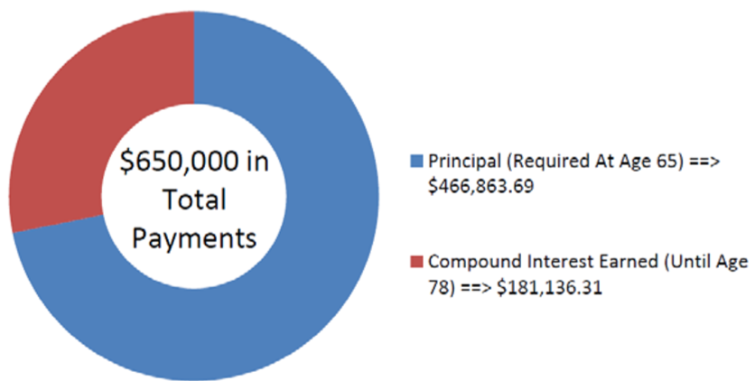
The figure shows how much principal and interest make up the payments. Rodriguez will need to have $466,863.69 in his account when he turns 65 if he wants to receive 13 years of $50,000 payments.
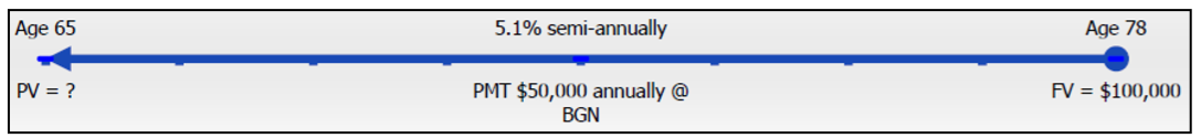
Recalculate Example \(\PageIndex{1}\) applying three changes:
- Rodriguez wants to leave a $100,000 inheritance for his children (assuming he dies at age 78).
- Payments are at the beginning of the year.
- His interest rate is 5.1% compounded semi-annually.
Calculate the present value and the amount of interest.
Solution
Step 1:
The payments are made at the beginning of the payment intervals, and the compounding period (semiannually) and payment intervals (annually) are different. This is now a general annuity due. Calculate its value at the start, which is its present value, or \(PV_{DUE}\).
What You Already Know
Step 1 (continued):
The timeline for the client's account appears below.
Step 2:
\(FV\) = $100,000, \(IY\) = 5.1%, \(CY\) = 2, \(PMT\) = $50,000, \(PY\) = 1, Years = 13
How You Will Get There
Step 3:
Apply Formula 9.1.
Step 4:
Since there is a future value, apply Formula 9.2 and Formula 9.3.
Step 5:
Apply Formula 11.4 and Formula 11.5.
Step 6:
To calculate the interest, apply and adapt Formula 8.3, where \(FV = N × PMT + FV\) and \(I = FV − PV\)
Perform
Step 3:
\(i=5.1 \% \div 2=2.55 \%\)
Step 4:
\(N=2 \times 13=26\) compounds
\[\begin{aligned}\$ 100,000&=PV(1+0.0255)^{26} \\ PV&=\$ 100,000 \div 1.0255^{26}\\ &=\$ 51,960.42776\end{aligned} \nonumber \]
Step 5:
\(N=1 \times 13=13\) payments
\[\begin{aligned}PV_{DUE}&=\$ 50,000\left[\dfrac{1-\left[\frac{1}{(1+0.0255)^{\frac{2}{1}}}\right]^{13}}{(1+0.0255)^{\frac{2}{1}}-1}\right] \times(1+0.0255)^{\frac{2}{1}}\\ &=\$ 489,066.6372 \end{aligned} \nonumber \]
\[PV=\$ 51,960.42776+\$ 489,066.6372=\$ 541,027.07 \nonumber \]
Step 6:
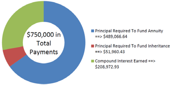
\[\begin{aligned}I&=(13 \times \$ 50,000+\$ 100,000)-\$ 541,027.07 \\ I&=\$ 750,000-\$ 541,027.07\\ &=\$ 208,972.93 \end{aligned} \nonumber \]
Calculator Instructions
| Mode | N | I/Y | PV | PMT | FV | P/Y | C/Y |
|---|---|---|---|---|---|---|---|
| BGN | 13 | 5.1 | Answer: -541,027.065 | 50000 | 100000 | 1 | 2 |
The figure shows how much principal and interest make up the payments.Rodriguez will require more money, needing to have $541,027.07 in his account when he turns 65 if he wants to receive 13 years of $50,000 payments while leaving a $100,000 inheritance for his children. His account will earn $208,972.93 over the time frame.
Important Notes
If any of the variables, including \(IY, CY, PMT\), or \(PY\), change between the start and end point of the annuity, or if any additional single payment deposit or withdrawal is made, this creates a new time segment that you must treat separately. There will then be multiple time segments that require you to work from right to left by repeating steps 3 through 5 in the procedure. Remember that the present value at the beginning of one time segment becomes the future value at the end of the next time segment. Example \(\PageIndex{3}\) illustrates this concept.
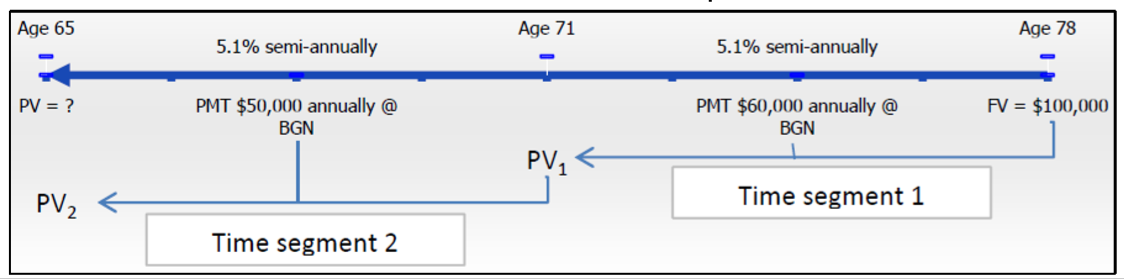
Continuing with the previous two examples, Rodriguez realizes that during his retirement he needs to make some type of adjustment to his annual gross income to account for the rising cost of living. Consequently, he will take $50,000 at the beginning of each year for six years, then increase it to $60,000 for the balance. Assume his interest rate is still 5.1% semiannually and that he still wants to leave a $100,000 inheritance for his children. How much money needs to be in his retirement fund at age 65?
Solution
Step 1:
There is a change of variables after six years. As a result, you need two time segments. In both segments, payments are made at the beginning of the period, and the compounding periods and payment intervals are different. These are two consecutive general annuities due. You need to calculate the resulting present value, or \(PV_{DUE}\).
What You Already Know
Step 1 (continued):
The timeline for the client's account appears below.
Step 2:
Time segment 1 (starting from the right side): \(FV\) = $100,000, \(IY\) = 5.1%, \(CY\) = 2, \(PMT\) = $60,000, \(PY\) = 1, Years = 7
Time segment 2: \(FV = PV_1\) of time segment 1, \(IY\) = 5.1%, \(CY\) = 2, \(PMT\) = $50 000, \(PY\) = 1, Years = 6
How You Will Get
There For each time segment repeat the following steps:
Step 3:
Apply Formula 9.1.
Step 4:
Apply Formula 9.2 and Formula 9.3.
Step 5:
Apply Formula 11.1 and Formula 11.5.
Perform
For the first time segment (starting at the right side):
Step 3:
\(i=5.1 \% \div 2=2.55 \%\)
Step 4:
\(N=2 \times 7=14\) compounds
\[\$ 100,000=PV(1+0.0255)^{14} \nonumber \]
\[PV_1=5100,000 \div 1.0255^{14}=\$ 70,291.15736 \nonumber \]
Step 5:
\(N=1 \times 7=7\) payments
\[PV_{DUE 1}=\$ 60,000\left[\dfrac{1-\left[\frac{1}{(1+0.0255)^{\frac{2}{1}}}\right]^{7}}{(1+0.0255)^{\frac{2}{1}}-1}\right] \times(1+0.0255)^{\frac{2}{1}}=\$ 362,940.8778 \nonumber \]
\[\text { Total } PV_1=\$ 70,291.15736+\$ 362,940.8778=\$ 433,232.0352 \nonumber \]
For the second time segment:
Step 3:
\(i\) remains the same = 2.55%
Step 4:
\(N=2 \times 6=12\) compounds
\[\$ 433,232.0352=PV(1+0.0255)^{12}\nonumber \]
\[PV_{2}=\$433,232.0352 \div 1.0255^{12}=\$ 320,252.5426 \nonumber \]
Step 5:
\(N=1 \times 6=6 \) payments
\[PV_{DUE 2}=\$ 50,000\left[\dfrac{1-\left[\frac{1}{(1+0.0255)^{\frac{2}{1}}}\right]^{6}}{(1+0.0255)^{\frac{2}{1}}-1}\right] \times(1+0.0255)^{\frac{2}{1}}=\$ 265,489.8749 \nonumber \]
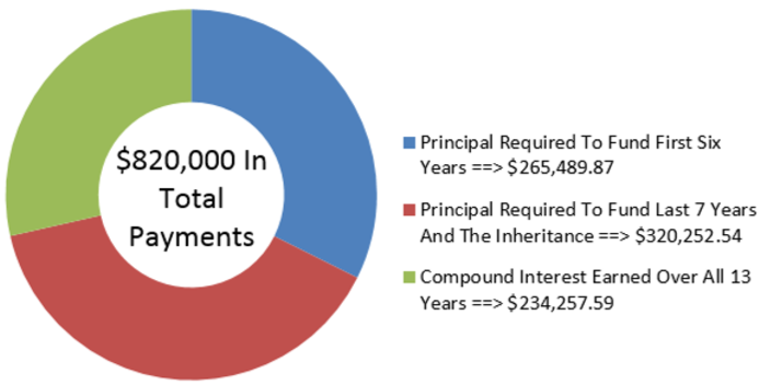
\[\text { Total } PV_{2}=\$ 320,252.5426+\$ 265,489.8749=\$ 585,742.42 \nonumber \]
Calculator Instructions
| Time Segment | Mode | N | I/Y | PV | PMT | FV | P/Y | C/Y |
|---|---|---|---|---|---|---|---|---|
| 1 | BGN | 7 | 5.1 | Answer: -433,232.0352 | 60000 | 100000 | 1 | 2 |
| 2 | \(\surd\) | 6 | \(\surd\) | Answer: -585,742.4175 | 50000 | 433,232.0352 | \(\surd\) | \(\surd\) |
The figure shows how much principal and interest make up the payments. To have his retirement income increased by $10,000 after six years, Rodriguez needs to have $585,742.42 invested in his retirement fund at age 65.
Working with Loans
At the start of this chapter, you purchased your first home and started your $150,000 mortgage at 5% compounded semi-annually. Assume your mortgage has a five-year term. Before that term expires, you have to start shopping around at different financial institutions to find the best rate for your next mortgage term. These other financial institutions will have one burning question: How much do you still owe on your mortgage and, thus, how much do you need to borrow from them?
Up to this point, this chapter has addressed only the concept of investment annuities. But what about debts? All annuity concepts also apply to the borrowing of money. When you work with loans, both future value and present value calculations may be required, which is why this topic has been delayed to this point.
As a consumer, you are probably most interested in the balance owing on any of your debts at any given point. Today's technology has made it easy to know your current balance by visiting your online bank account; however, the bank account does not assist you in identifying your future balance at a given point in time. To figure this out, you need annuity calculations.
Similarly, businesses apply annuity calculations all the time. Ongoing financial reporting has to be accurate. To provide insight into the company's true financial health, balance sheets need to reflect not only monies payable or receivable today, but also all future cash flows such as those arising from annuities. The purchase and sale of business contracts, such as the sale of a consumer payment plan to a financial institution, requires working with future payments and discounting those payments to the contract's date of sale.
In this section, you will calculate loan balances at any given point in time throughout the loan's term. As well, you will explore how to buy and sell loan contracts.
The Balance Owing on Any Loan Contract
To determine accurately the balance owing on any loan at any point in time, always start with the loan's starting principal and then deduct the payments made. This means a future value calculation using the loan's interest rate.
Some may ask why they can't figure out the loan balance by starting at the end of the loan (where the future value is zero, since no balance remains) and calculating a present value of the outstanding payments? The answer is because the annuity payment \(PMT\) is almost always a rounded number (this characteristic is explored in greater depth in Section 11.4, when you learn how to calculate the annuity payment). Every payment therefore has a slight discrepancy from its true value, which accumulates with each subsequent payment. For example, assume you calculate your payment mathematically as $500.0045. Since you can't pay more than two decimals, your actual payments are $500.00. The $0.0045 is dropped, which means every payment you make is $0.0045 short of what is mathematically required. If you make 100 such payments, the $0.0045 error accumulates to $0.45 plus interest. This means your very last payment must be increased by $0.45 or more to pay off your loan. Thus, the last payment is a different amount than every other payment.
To complicate matters further, the last payment amount may be unknown and incalculable, particularly if interest rates are variable. You can't calculate a present value from an unknown number nor can you use an annuity formula where a payment is in a different amount. Chapter 13 provides much more detail about these concepts of loan payments, loan balances, and final payment differences. For now, you can conclude that an accurate calculation of a loan balance is achieved through a future value annuity formula.
The Formula
Loans are most commonly ordinary annuities requiring the application of Formula 11.2 (ordinary annuity future value) to calculate the future balance, \(FV_{ORD}\). This is the basic assumption in performing loan calculations unless otherwise specified. In the rare instance of a loan structured as an annuity due, you apply Formula 11.3 (annuity due future value) to calculate the future value, \(FV_{DUE)\).
Calculating the total amount of interest paid on a loan (in whole or for any time segment) once again requires the adaptation of Formula 8.3 (\(I = S – P = FV − PV\)), where:
- The future value (\(FV\)) term in the formula represents the total principal and interest combined. In loan annuities, the annuity payment incorporates both of these elements. As well, any future principal remaining at the end of the loan, or a future balance outstanding, must also be factored into the calculation. Hence, the \(FV\) at any time interval in the formula is expanded to include both of these elements and replaced by \(N × PMT + FV\).
- The present value (\(PV\)) in the formula is what you started with. It is the opening amount of the loan. Therefore, the adaptation of Formula 8.3 remains the same as previously discussed and is written as: \[I = (N × PMT + FV) − PV \nonumber \].
How It Works
Solving for a future loan balance is a future value annuity calculation. Therefore, you use the same steps as discussed in Section 11.2. However, you need to modify your interpretation of these steps for loan balances. The figure below helps you understand these differences.
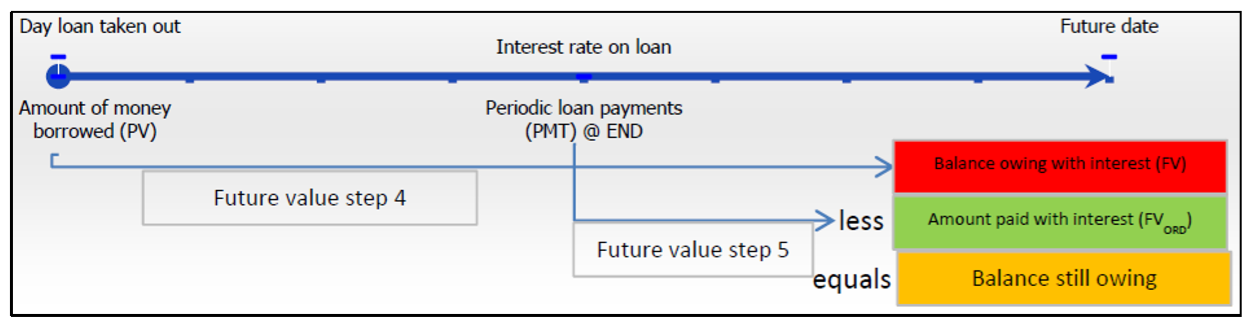
- The principal of the loan forms the present value, or \(PV\). In step 4, when you move the present value to the future, your answer (\(FV\)) represents the total amount owing on the loan with interest as if no payments had been made.
- In step 5, the future value of the annuity (\(FV_{ORD}\)) represents the total amount paid against the loan with interest. With both the \(FV\) and \(FV_{ORD}\) on the same focal date, the fundamental concept of the time value of money allows you to then take the \(FV\) and subtract the \(FV_{ORD}\) to produce the balance owing on the loan.
Let’s calculate what you still owe on your $150,000 new home after five years of making $872.41 monthly payments at 5% compounded semi-annually:
Step 1: The structure of your mortgage is depicted in the Figure above. Since payments are at the end of the period, and the payment interval and compounding frequency are different, you have an ordinary general annuity.
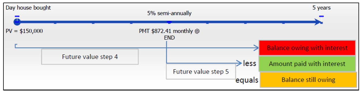
Step 2: The known variables are \(PV\) = $150,000, \(IY\) = 5%, \(CY\) = 2, \(PMT\) = $872.41, \(PY\) = 12, and Years = 5.
Step 3: The periodic interest rate is \(i\) = 5% ÷ 2 = 2.5%.
Step 4: \(N\) = 2 × 5 = 10 compounds, \(FV\) = $150,000(1 + 0.025)10 = $192,012.6816
Step 5: \(N\) = 12 × 5 = 60 payments
\[FV_{ORD}=\$ 872.41\left[\dfrac{\left[(1+0.025)^{\frac{2}{12}}\right]^{60}-1}{(1+0.025)^{\frac{2}{12}}-1}\right]=\$ 59,251.59215 \nonumber \]
Therefore, if the unpaid loan is worth $192,012.6816 and your payments are worth $59,251.59215, then your balance still owing is $192,012.6816 − $59,251.59215 = $132,761.09. The amount of interest paid is I = (60 × $872.41 + $132,761.09) − $150,000.00 = $35,105.69. With payments totaling $872.41 × 60 = $52,344.60, that means only $17,238.91 actually went towards the principal!
Important Notes
Present Value Method of Arriving at a Balance Owing. In the rare circumstance where the final payment is exactly equal to all other annuity payments, you can arrive at the balance owing through a present value annuity calculation. However, this strict condition must be met. In this instance, since you are starting at the end of the loan, the future value is always zero, so to bring all payments back to the focal date you only need Formula 11.4.
Your BAII+ Calculator. Proper application of the cash flow sign convention for the present value and annuity payment will automatically result in a future value that nets out the loan principal and the payments. Assuming you are the borrower, you enter the present value (\(PV\)) as a positive number since you are receiving the money. You enter the annuity payment (\(PMT\)) as a negative number since you are paying the money. When you calculate the future value (\(FV\)), it displays a negative number, indicating that it is a balance owing.
On any interest-bearing loan at any point in time, will the principal be reduced by an amount equal to the payments made, more than the payments made, or less than the payments made?
- Answer
-
The principal will be reduced by an amount less than the payments. A portion of the payments always goes toward the interest that is being charged on the loan.
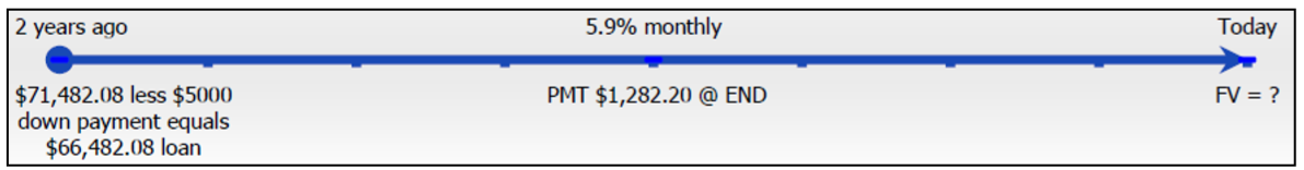
Two years ago, Jillian purchased a new Ford F-250 for $71,482.08 with a $5,000 down payment and the remainder financed through her Ford dealership at 5.9% compounded monthly. She has been making monthly payments of $1,282.20. What is her balance owing today? How much interest has she paid to date?
Solution
Step 1:
The payments are made at the end of the payment intervals, and the compounding period and payment intervals are the same. Therefore, this is a simple ordinary annuity. Calculate its value two years after its start, which is its future value, or \(FV_{ORD}\). Once you know the \(FV_{ORD}\), you can determine the amount of interest, or \(I\).
What You Already Know
Step 1 (continued):
The timeline for the savings annuity appears below.
Step 2:
\(PV\) = $71,482.08 − $5,000 = $66,482.08, \(IY\) = 5.9%, \(CY\) = 12, \(PMT\) = $1,282.20, \(PY\) = 12, Years = 2
How You Will Get There
Step 3:
Apply Formula 9.1.
Step 4:
Apply Formula 9.2 and Formula 9.3.
Step 5:
Apply Formula 11.1 and Formula 11.2. The final future value is the difference between the answers to step 4 and step 5.
Step 6:
To calculate the interest, apply the adapted Formula 8.3, where \(I = (N × PMT + FV) − PV\).
Step 3:
\[i=5.9 \% \div 12=0.491\overline{6} \% \nonumber \]
Step 4:
\(N=12 \times 2=24\) compounds
\[FV=\$ 66,482.08(1+0.00491\overline{6})^{24}=\$ 74,786.94231 \nonumber \]
Step 5:
\(N=12 \times 2=24\) payments
\[FV_{ORD}=\$ 1,282.20\left[\dfrac{\left.(1+0.00491 \overline{6})^{\frac{12}{12}}\right]^{24}-1}{(1+0.00491 \overline{6})^{\frac{12}{12}}-1}\right]=\$ 32,577.13179 \nonumber \]
\[FV=\$ 74,786.94231-\$ 32,577.13179=\$ 42,209.81 \nonumber \]
Step 6:
\[\begin{aligned} I &=(24 \times \$ 1,282.20+\$ 42,209.81)-\$ 66,482.08 \\ &=\$ 72,982.61-\$ 66,482.08\\ &=\$ 6,500.53 \end{aligned} \nonumber \]
Calculator Instructions
| N | I/Y | PV | PMT | FV | P/Y | C/Y |
|---|---|---|---|---|---|---|
| 24 | 5.9 | 66482.08 | -1282.2 | Answer: -42,209.81052 | 12 | 12 |
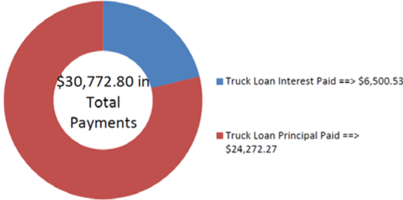
The figure shows how much principal and interest make up the payments. After two years of making monthly payments, Jillian has a balance owing on the Ford F-250 of $42,209.81. Altogether, she has made $30,772.80 in payments, of which $6,500.53 went toward the interest on her loan.
Selling a Loan Contract
It is common for loan contracts to be sold from retailers to financial institutions. For example, when a consumer makes a purchase from Sleep Country Canada on its payment plan, the financing is actually performed through its partner Citi Financial. In most retail situations, this would then mean that Sleep Country Canada receives the money right away by selling the contract to Citi Financial, whereas Citi Financial assumes the financial responsibility of collecting the payments.
When a finance company purchases a loan contract from another organization, it is essentially investing in the future payments of the loan contract. The two companies commonly agree on a profitable interest rate for the finance company and use it to determine the amount, known as the sale price, paid by the finance company to the other organization to purchase the contract. This textbook covers only fixed interest rate calculations with known final payment amounts.
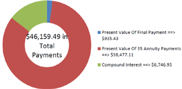
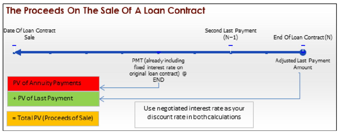
Previously, it was discussed how the last payment in a loan almost always differs from every other payment in the annuity because of the rounding discrepancy in the annuity payment amount. Thus, the selling of a loan contract needs to calculate the present value of all remaining annuity payments (except for the last one) plus the present value of the adjusted single final payment as shown in this figure.
The Formula
As evident in the figure, two calculations are required. The first involves a present value annuity calculation using Formula 11.4. Note that the annuity stops one payment short of the end of the loan contract, so you need to use \(N − 1\) rather than \(N\). The second calculation involves a present-value single payment calculation at a fixed rate using Formula 9.3 rearranged for \(PV\). Thus, no new formulas are required to complete this calculation.
How It Works
The steps involved in selling any loan contract are almost identical to any present value annuity calculation with only minor differences as noted below.
Step 1: No changes.
Step 2: Identify the known variables, including \(PMT, PY\), and Years, along with the newly negotiated \(IY\) and \(CY\). Also identify the amount of the last payment, which is the \(FV\).
Step 3: Use Formula 9.1 to calculate \(i\).
Step 4: The last payment is the \(FV\), which you treat like a single payment. Apply Formula 9.2 to determine \(N\) since this step is not an annuity calculation. Move the future value to the beginning of the time segment using Formula 9.3, rearranging for \(PV\).
Step 5: Use Formula 11.1 to calculate \(N\) and subtract 1 to remove the final payment (since it is accounted for in step 4). Apply Formula 11.4 (or Formula 11.5 if it is an annuity due) to calculate the present value. Add both of the present values from steps 4 and 5 together to arrive at the total present value, which is known as the total proceeds of the sale.
Continuing with Jillian's Ford F-250 purchase, recall that Jillian's monthly payments are fixed at $1,282.20 for five years. Assume that after two years Ford wants to sell the contract to another finance company, which agrees to a discount rate of 10.8% compounded semi-annually. Jillian's final payment is known at $1,282.49. What are the proceeds of the sale?
Solution
Step 1:
The payments are made at the end of the payment intervals, and the compounding period (semi-annually) and payment intervals (monthly) are different. Therefore, this is an ordinary general annuity. Calculate its value on the date of sale, which is its present value, or \(PV_{DUE}\), plus the present value of the final payment, or \(PV\).
What You Already Know
Step 1 (continued):
The timeline for the sale of the loan contract appears below.
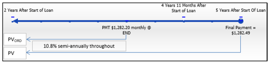
Step 2: \(FV\) = $1,282.49, \(IY\) = 10.8%, \(CY\) = 2, \(PMT\) = $1,282.20, \(PY\) = 12, Years = 3
How You Will Get There
Step 3:
Apply Formula 9.1.
Step 4:
For the final payment amount, apply Formula 9.2 and Formula 9.3, rearranging for \(PV\).
Step 5:
For the annuity, apply Formula 11.1 (taking away the last payment) and Formula 11.4.
Perform
Step 3:
\[i=10.8 \% \div 2=5.4 \% \nonumber \]
Step 4:
\(N=2 \times 3=6\) compounds
\[\$ 1,282.49=PV(1+0.054)^{6} \nonumber \]
\[PV=\$ 1,282.49 \div 1.054^{6}=\$ 935.427906 \nonumber \]
Step 5:
\(N=12 \times 3-1=35 \) payments
\[PV_{ORD}=\$ 1,282.20\left[\dfrac{1-\left[\frac{1}{(1+0.054)^{\frac{2}{12}}}\right]^{35}}{(1+0.054)^{\frac{2}{12}}-1}\right]=\$ 38,477.10711 \nonumber \]
\[PV=\$ 935.427906+\$ 38,477.10711=\$ 39,412.54 \nonumber \]
Calculator Instructions
| Element | N | I/Y | PV | PMT | FV | P/Y | C/Y |
|---|---|---|---|---|---|---|---|
| Final Payment | 6 | 10.8 | Answer: -935.427906 | 0 | 1282.49 | 2 | 2 |
| Annuity | 35 | \(\surd\) | Answer: -38,477.10711 | 1282.2 | 0 | 12 | 2 |
The figure shows the present value and interest amounts in the transaction. The finance company will pay $39,412.54 for the contract. In return, it receives 35 payments of $1,282.20 and one payment of $1,282.49 for a nominal total of $46,159.49.