12.2: Constant-Growth Annuities
- Page ID
- 22139

Many experts recommend that you should save around 10% of your annual income toward your RRSP contributions. Like most people, when you graduate college or university, your employer will offer you a starting salary that is usually at the lower end of their pay scale. In most companies, you are then eligible to receive annual raises in accordance with a predetermined pay structure or through performance reviews. This represents an annual income that always rises. As a result, your RRSP contributions should always rise annually too.
All annuity calculations so far have permitted fixed contributions only. More realistically, in many financial situations, such as your RRSP, the annuity payments should constantly increase on a regular basis. For this situation you need to study constant growth annuities.
The Concept of Constant Growth
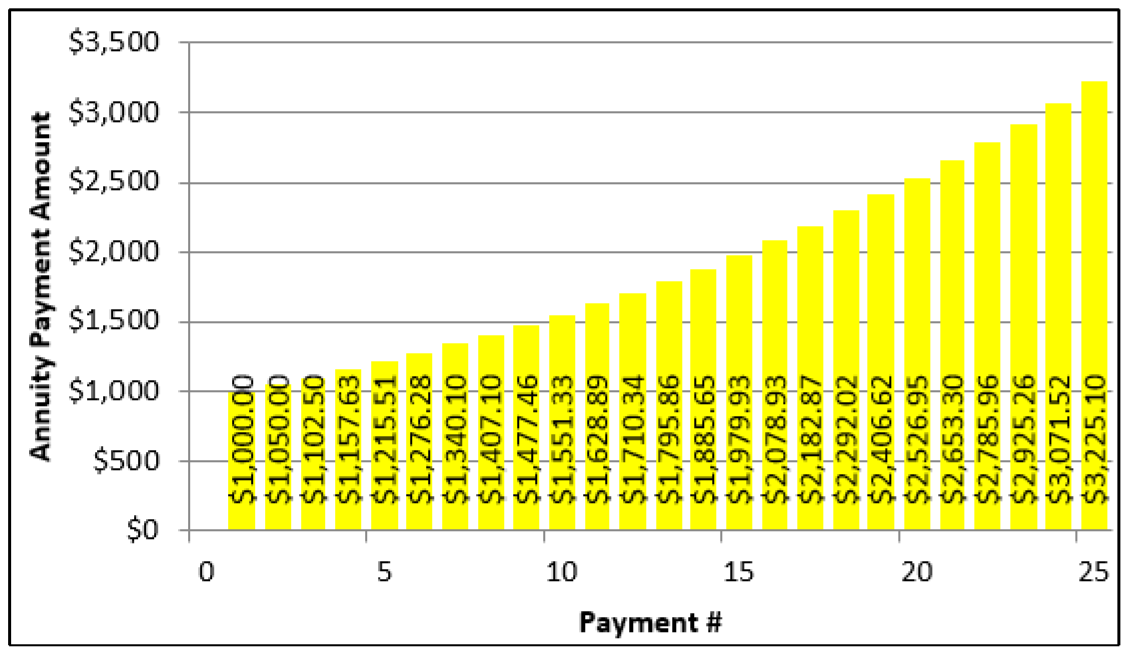
A constant growth annuity is an annuity in which each annuity payment is increased by a fixed percentage. The figure here illustrates a $1,000 initial payment growing by 5% with each subsequent payment.
In addition to your RRSP contributions, annuity payments are regularly increased in many situations:
- When you draw from your retirement savings, you must increase your payments each year to keep up with the cost of living. This increasing demand on your retirement fund must be factored into a proper RRSP savings plan.
- Payments by the Canada Pension Plan and Old Age Security, along with most private company pension plans, increase annually to match the rate of inflation.
The change in each payment is a fixed percentage and therefore represents a percent change in the annuity payment. This can be represented by the percent change symbol, \(∆\%\), used in Section 3.1. This variable represents the periodic percent change, where the period is consistent with the payment interval. Thus, if the payments are monthly then the percent change variable needs to be expressed as the percent change per month.
The Impact of Constant Growth on the Annuity Payment
To understand how constant growth affects the annuity payment variable, take a look at how the first four payments in any constant growth annuity are represented. Recall in annuities that \(N\) represents the number of payments, therefore:
\(N = 1\): First payment \(= PMT = PMT(1 + ∆\%)^{N – 1}\) (since \(N = 1\), this produces a zero exponent on the percent change)
\(N = 2\): Second payment \(= PMT (1 + ∆\%) = PMT(1 + ∆\%)^{N – 1}\)
\(N = 3\): Third payment \(= PMT (1 + ∆\%)(1 + ∆\%) = PMT (1 + ∆\%)^2 = PMT(1 + ∆\%)^{N – 1}\)
\(N = 4\): Fourth payment \(= PMT (1 + ∆\%)(1 + ∆\%)(1 + ∆\%) = PMT (1 + ∆\%)^3 = PMT(1 + ∆\%)^{N – 1}\)
Notice that every annuity payment ultimately is represented by \(PMT(1 + ∆\%)^{N – 1}\) regardless of the number of annuity payments made.
The Impact of Constant Growth on the Annuity Interest Rate
You must adjust the annuity periodic interest rate to isolate the growth in the annuity from interest, since the growth in the annuity payments is already reflected in the \(PMT(1 + ∆\%)^{N – 1}\) above. Over the course of any single period, interest compounds at a rate calculated as \(1 + i\). On the other hand, contributions over the same time period grow by \(1 + ∆\%\). Therefore, the interest in the account grows more than the growth in the contributions by a rate that is calculated by:
\[\dfrac{(1+i)}{(1+\Delta \%)}-1 \nonumber \]
For illustrative purposes, assume an annuity with a periodic interest rate of 10% and a periodic growth rate of 5%. Apply the above calculation:
\[\dfrac{1+0.1}{1+0.05}-1=\dfrac{1.1}{1.05}-1=0.047619 \nonumber \]
Therefore, each period the net growth attributable solely to interest represents a periodic compounding of 4.7619% and not 10%. This interest rate, sometimes called the net rate, must replace the periodic interest rate you use in all annuity formulas.
The Formula
The four formulas for the future value and present value of both ordinary and annuity dues are shown below, incorporating the concept of constant growth. Notice in every formula that the periodic interest rate is changed to net rate. The percent change formula in the denominator does not require the \(\dfrac{CY}{PY}\) exponent since the variable is already expressed in the same periodic terms as the payments.
- Future Value Formulas. The annuity payment is modified to incorporate the growth in the payments from \(PMT\) to \(PMT(1 + ∆\%)^{N – 1}\) as previously illustrated. The first payment has zero growth, which results in an exponent having one period of growth less than the number of payments made.
- Present Value Formulas. When bringing the annuity back to its beginning, this represents the 0th payment since a first payment has not occurred yet. Applying the \(PMT(1 + ∆\%)^{N – 1}\) formula results in \(PMT(1+\Delta \%)^{0-1}=PMT(1+\Delta \%)^{-1}=\dfrac{PMT}{1+\Delta \%}\), which then substitutes for \(PMT\) in the formula.
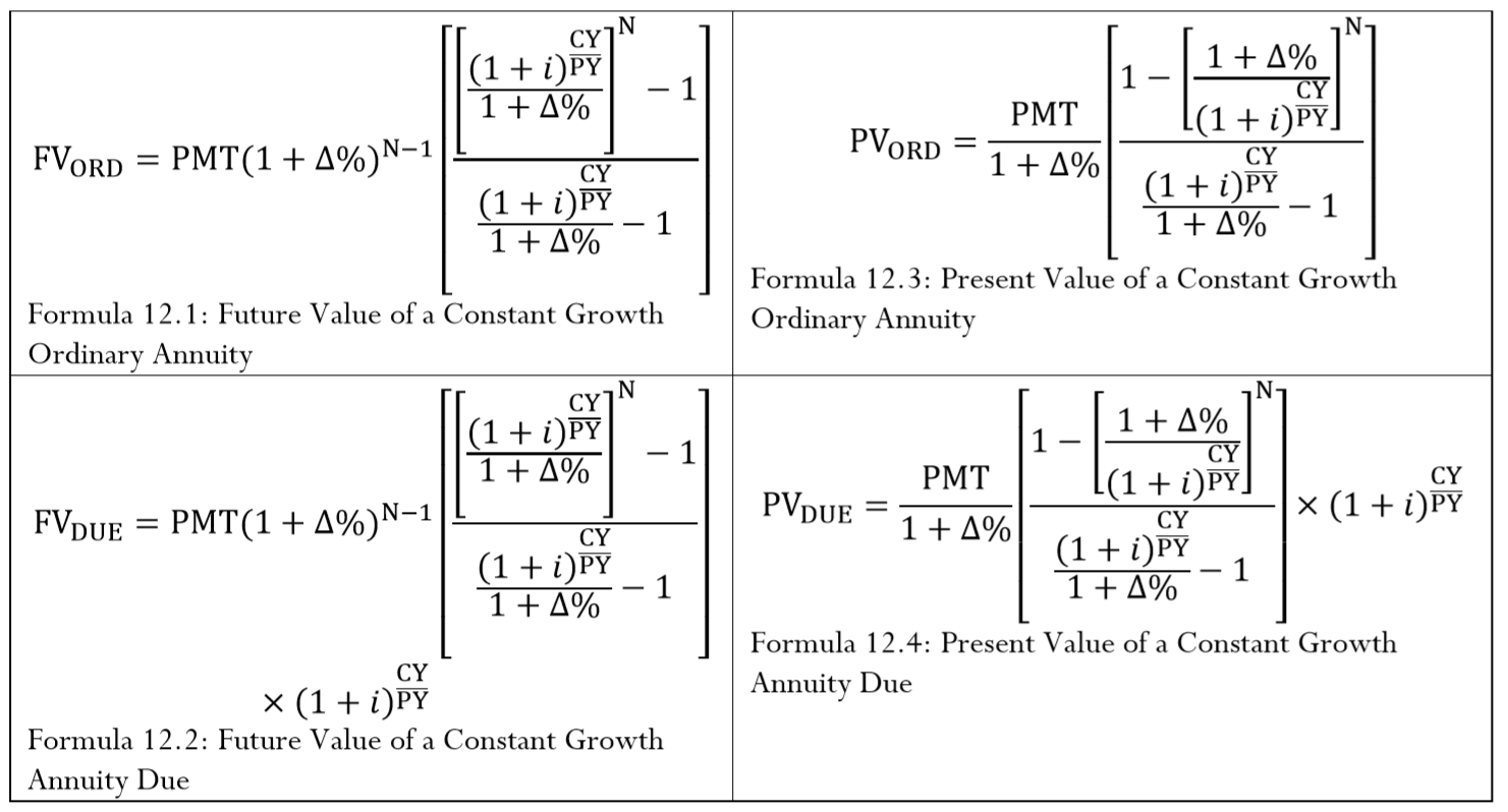
Formula for Future Value and Growth Value - 12.1, 12.2, 12.3, 12.4
Make the following notes about the variables:
- \(PMT\). Every payment is constantly increasing in a constant growth annuity. Therefore, the first payment is the clearly identifiable value. To ascertain the value of any other payment, use the formula \(PMT(1+\Delta \%)^{N-1}\), as illustrated previously. For example, if a $1,000 payment is growing at 5% and the value of the 10th payment needs to be known, it is calculated as \(\$ 1,000(1+0.05)^{10-1}=\$ 1,551.33\).
- \(i\). The rate of interest resulting from Formula 9.1, converted to match the payment interval if necessary. The periodic interest rate is adjusted to reflect the net rate by dividing it by \(1 + ∆\%\).
- \(∆\%\). The periodic percent change matching the payment interval between each successive payment in the annuity. If payments are made quarterly, then the percent change per quarter is required. The value of \(∆\%\) in these formulas is restricted to a value less than the equivalent periodic interest rate \(i\) (where \(i\) is expressed as the interest rate per payment interval). Situations where \(\Delta \% \geq(1+i)^{\frac{CY}{PY}}-1\) are beyond the scope of this textbook. If \(∆\%\) is assigned a value of 0% then these formulas revert back to Formulas 11.2 to 11.5, respectively. Hence, the formulas from Chapter 11 are sometimes referred to as zero growth annuity formulas and represent simplified versions of these complete annuity formulas.
How It Works
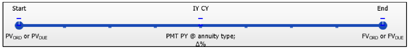
Follow the same steps discussed for future value in Section 11.2 and the steps for present value in Section 11.3. The only notable difference is that you must identify the periodic growth rate for the annuity payment and, of course, use the new Formulas 12.1 to 12.4. The figure below illustrates a typical timeline when constant growth is involved. Note the \(∆\%\) after the annuity type and that only one of \(FV_{ORD}\), \(FV_{DUE}\), \(PV_{ORD}\), or \(PV_{DUE}\) ever appears on the timeline.
The most common applications involving constant growth annuities require you to calculate the future value, present value, or the first annuity payment. In the first two cases, you use Formulas 12.1 to 12.4 to solve for \(FV\) and \(PV\). If the first annuity payment is the unknown variable, you can rearrange any of Formulas 12.1 to 12.4 algebraically to isolate \(PMT\) as needed.
Important Notes
Most financial calculators, including the Texas Instruments BAII Plus, are not pre-programmed with constant growth annuities. They are designed to handle fixed payment annuities only.
That said, on the web or in your readings you may come across methods that show you how to adapt your calculator input to "trick" the calculator. It is important to note that these methods are generally complex, requiring you to memorize a lot of adaptations and conditional modifications. Outputs are not necessarily correct unless further adapted. Ultimately, these tricks are not recommended. This textbook solves constant growth annuities only using formulas and through the Excel template.
Paths To Success
Although all of the discussion has been about growth, you can also use these formulas in situations involving constant reduction since the requirement of \(\Delta \%<(1+i)^{\frac{CY}{PY}}-1\) remains true. Use a negative value for the growth rate in all calculations.
Additionally, if you wish to know the total value of the annuity payments in a constant growth annuity, you can use Formula 11.2 with a few adaptations:
- Treat the first payment as the annuity payment amount or \(PMT\).
- Substitute the periodic growth rate for the equivalent periodic interest rate while setting \(CY\) and \(PY\) both to 1. This eliminates the \(\dfrac{CY}{PY}\) exponent.
- Retain using \(N\) as the number of payments.
Thus, substituting and simplifying produces the following calculation:
\[\text { Sum of constant growth payments }=PMT\left[\dfrac{[(1+\Delta \%)]^{\mathrm{N}}-1}{\Delta \%}\right] \nonumber \]
If an annuity payment is increased by $5 each time from $100 to $105 to $110 to $115, does this represent a situation of constant growth?
- Answer
-
No. A constant growth is represented by a fixed percentage growth, not a fixed dollar amount growth.
Bradford is 27 years old and starts investing $3,000 per year into his RRSP earning 9% compounded annually. He decides that each year he will increase his contributions by 2.5%. Calculate the maturity value at age 65 for both an ordinary annuity and an annuity due.
Solution
If every payment is increasing by a fixed percentage, then this is a constant growth annuity. Calculate two maturity values, one for the ordinary annuity, or \(FV_{ORD}\), and one for the annuity due, or \(FV_{DUE}\).
What You Already Know
Step 1:
There are annual contributions with an annual compound interest rate. The beginning payment creates a simple constant growth annuity due, while the end payments create an ordinary simple constant growth annuity. The timeline is below.
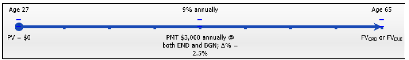
Step 2:
Both annuities: \(PV\) = $0, \(IY\) = 9%, \(CY\) = 1, \(PMT\) = $3,000, \(PY\) = 1, Years = 38, \(∆\%\) = 2.5%
How You Will Get There
Step 3:
Apply Formula 9.1.
Step 4:
With \(PV\) = $0, skip this step.
Step 5:
Apply Formula 11.1 and Formulas 12.1 and 12.2.
Perform
Step 3:
\(i=9 \% / 1=9 \%\)
Step 5:
\(N=1 \times 38=38 \text { payments } \)
\[FV_{ORD}=\$ 3,000(1+0.025)^{37}\left[\dfrac{\left [\dfrac{(1+0.09)^{\frac{1}{1}}}{(1+0.025)^{\frac{1}{1}}} \right ]^{38}-1}{\dfrac{(1+0.09)^{\frac{1}{1}}}{(1+0.025)^{\frac{1}{1}}}-1}\right]=\$ 1,102,199.91 \nonumber \]
\[FV_{DUE}=\$ 1,102,199.91 \times(1+0.09)^{\frac{1}{1}}=\$ 1,201,397.90 \nonumber \]
The 38 contributions amount to a total principal contribution of $186,681.89. The maturity value of the ordinary annuity is $1,102,199.91 and the annuity due is one compound higher at $1,201,397.90.
How much money is required today to fund a 10-year annuity earning 5.6% compounded quarterly where the first monthly payment will be $2,000 and each payment will grow by 0.2%? Calculate as both an ordinary annuity and annuity due.
Solution
If every payment is increasing by a fixed percentage, then this is a constant growth annuity. Calculate two principal amounts, one for the ordinary annuity, or \(PV_{ORD}\), and one for the annuity due, or \(PV_{DUE}\).
What You Already Know
Step 1:
There are monthly payments with a quarterly compound interest rate. The beginning payments create a general constant growth annuity due, while the end payments create an ordinary general constant growth annuity.
The timeline appears below.
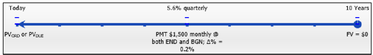
Step 2:
Both annuities: \(FV\) = $0, \(IY\) = 5.6%, \(CY\) = 4, \(PMT\) = $2,000, \(PY\) = 12, Years = 10, \(∆\%\) = 0.2%
How You Will Get There
Step 3:
Apply Formula 9.1.
Step 4:
With \(FV\) = $0, skip this step.
Step 5:
Apply Formula 11.1 and Formulas 12.3 and 12.4.
Perform
Step 3:
\(i=5.6 \% / 4=1.4 \%\)
Step 5:
\(N=12 \times 10=120 \text { payments } \)
\[ PV_{ORD}=\dfrac{\$ 2,000}{1+0.002}\left[\dfrac{1-\left[\dfrac{(1+0.002)}{(1+0.014)^{\frac{4}{12}}}\right]^{120}}{\dfrac{(1+0.014)^{\frac{4}{12}}}{(1+0.002)}-1}\right]=\$ 205,061.74 \nonumber \]
\[PV_{DUE}=\$ 205,061.7409 \times(1+0.014)^{\frac{4}{12}}=\$ 205,061.7409 \times 1.004645=\$ 206,014.26 \nonumber \]
The 120 payments each increased by 0.2% amounts to a total payout of $270,944.49. To fund these payouts, an ordinary constant growth annuity requires $205,061.74 today, whereas a constant growth annuity due requires a little more, equaling $206,014.26 because the first payment is withdrawn immediately.
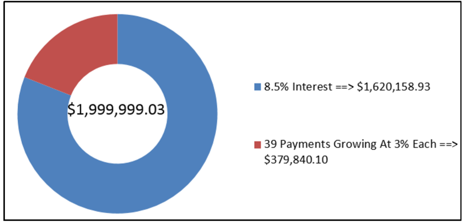
After a discussion with her financial adviser on February 28, 2012, Jennifer has determined that she needs $2 million in her RRSP when she retires on February 28, 2051. She has decided to start making annual contributions to her RRSP starting February 28, 2013, and grow those contributions by 3% every year. If her RRSP can earn 8.5% compounded annually, in what amount should she make her first contribution?
Solution
If every payment is increasing by a fixed percentage, then this is a constant growth annuity. Calculate the amount of her first annuity payment (\(PMT\)).
What You Already Know
Step 1:
There are annual contributions at the end of the interval with an annual compound interest rate. Therefore, this is an ordinary simple constant growth annuity.
The timeline appears below.
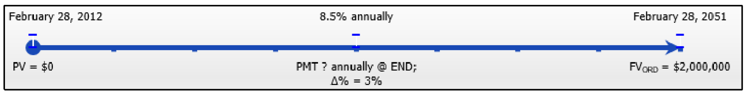
Step 2:
\(PV\) = $0, \(FV_{ORD}\) = $2,000,000, \(IY\) = 8.5%, \(CY\) = 1, \(PY\) = 1, Years = 39, \(∆\%\) = 3%
How You Will Get There
Step 3:
Apply Formula 9.1.
Step 4:
With \(PV\) = $0, skip this step.
Step 5:
Apply Formula 11.1 and Formula 12.1. Once you have substituted and simplified this formula, rearrange it for \(PMT\).
Step 3:
\(i=8.5 \% / 1=8.5 \%\)
Step 5:
\(N=1 \times 39=39 \text { payments } \)
\[\$ 2,000,000=PMT(1+0.03)^{38}\left[\dfrac{\left[\dfrac{(1+0.085)^{\frac{1}{3}}}{(1+0.05)^{\frac{1}{1}}}\right]^{39}-1}{\dfrac{(1+0.055)^{\frac{1}{1}}}{(1+0.03)^{\frac{1}{1}}}-1}\right] \nonumber \]
\[\$ 2,000,000=PMT(3.074783)\left[\dfrac{6.605154}{0.053398}\right] \nonumber \]
\[\begin{align*} \$ 2,000,000&=PMT(380.340030) \\ \$ 5,258.45&=PMT \end{align*} \nonumber \]
Jennifer's first payment is $5,258.45 and then increased by 3% each year for her 39 payments to provide enough principal to achieve her $2,000,000 financial goal. Note that because of the rounding of the first annuity payment, she in fact ends up marginally short of her goal in the amount of $0.97.