
15.7: Chapter 8
- Page ID
- 129937

\( \newcommand{\vecs}[1]{\overset { \scriptstyle \rightharpoonup} {\mathbf{#1}} } \)
\( \newcommand{\vecd}[1]{\overset{-\!-\!\rightharpoonup}{\vphantom{a}\smash {#1}}} \)
\( \newcommand{\dsum}{\displaystyle\sum\limits} \)
\( \newcommand{\dint}{\displaystyle\int\limits} \)
\( \newcommand{\dlim}{\displaystyle\lim\limits} \)
\( \newcommand{\id}{\mathrm{id}}\) \( \newcommand{\Span}{\mathrm{span}}\)
( \newcommand{\kernel}{\mathrm{null}\,}\) \( \newcommand{\range}{\mathrm{range}\,}\)
\( \newcommand{\RealPart}{\mathrm{Re}}\) \( \newcommand{\ImaginaryPart}{\mathrm{Im}}\)
\( \newcommand{\Argument}{\mathrm{Arg}}\) \( \newcommand{\norm}[1]{\| #1 \|}\)
\( \newcommand{\inner}[2]{\langle #1, #2 \rangle}\)
\( \newcommand{\Span}{\mathrm{span}}\)
\( \newcommand{\id}{\mathrm{id}}\)
\( \newcommand{\Span}{\mathrm{span}}\)
\( \newcommand{\kernel}{\mathrm{null}\,}\)
\( \newcommand{\range}{\mathrm{range}\,}\)
\( \newcommand{\RealPart}{\mathrm{Re}}\)
\( \newcommand{\ImaginaryPart}{\mathrm{Im}}\)
\( \newcommand{\Argument}{\mathrm{Arg}}\)
\( \newcommand{\norm}[1]{\| #1 \|}\)
\( \newcommand{\inner}[2]{\langle #1, #2 \rangle}\)
\( \newcommand{\Span}{\mathrm{span}}\) \( \newcommand{\AA}{\unicode[.8,0]{x212B}}\)
\( \newcommand{\vectorA}[1]{\vec{#1}} % arrow\)
\( \newcommand{\vectorAt}[1]{\vec{\text{#1}}} % arrow\)
\( \newcommand{\vectorB}[1]{\overset { \scriptstyle \rightharpoonup} {\mathbf{#1}} } \)
\( \newcommand{\vectorC}[1]{\textbf{#1}} \)
\( \newcommand{\vectorD}[1]{\overrightarrow{#1}} \)
\( \newcommand{\vectorDt}[1]{\overrightarrow{\text{#1}}} \)
\( \newcommand{\vectE}[1]{\overset{-\!-\!\rightharpoonup}{\vphantom{a}\smash{\mathbf {#1}}}} \)
\( \newcommand{\vecs}[1]{\overset { \scriptstyle \rightharpoonup} {\mathbf{#1}} } \)
\(\newcommand{\longvect}{\overrightarrow}\)
\( \newcommand{\vecd}[1]{\overset{-\!-\!\rightharpoonup}{\vphantom{a}\smash {#1}}} \)
\(\newcommand{\avec}{\mathbf a}\) \(\newcommand{\bvec}{\mathbf b}\) \(\newcommand{\cvec}{\mathbf c}\) \(\newcommand{\dvec}{\mathbf d}\) \(\newcommand{\dtil}{\widetilde{\mathbf d}}\) \(\newcommand{\evec}{\mathbf e}\) \(\newcommand{\fvec}{\mathbf f}\) \(\newcommand{\nvec}{\mathbf n}\) \(\newcommand{\pvec}{\mathbf p}\) \(\newcommand{\qvec}{\mathbf q}\) \(\newcommand{\svec}{\mathbf s}\) \(\newcommand{\tvec}{\mathbf t}\) \(\newcommand{\uvec}{\mathbf u}\) \(\newcommand{\vvec}{\mathbf v}\) \(\newcommand{\wvec}{\mathbf w}\) \(\newcommand{\xvec}{\mathbf x}\) \(\newcommand{\yvec}{\mathbf y}\) \(\newcommand{\zvec}{\mathbf z}\) \(\newcommand{\rvec}{\mathbf r}\) \(\newcommand{\mvec}{\mathbf m}\) \(\newcommand{\zerovec}{\mathbf 0}\) \(\newcommand{\onevec}{\mathbf 1}\) \(\newcommand{\real}{\mathbb R}\) \(\newcommand{\twovec}[2]{\left[\begin{array}{r}#1 \\ #2 \end{array}\right]}\) \(\newcommand{\ctwovec}[2]{\left[\begin{array}{c}#1 \\ #2 \end{array}\right]}\) \(\newcommand{\threevec}[3]{\left[\begin{array}{r}#1 \\ #2 \\ #3 \end{array}\right]}\) \(\newcommand{\cthreevec}[3]{\left[\begin{array}{c}#1 \\ #2 \\ #3 \end{array}\right]}\) \(\newcommand{\fourvec}[4]{\left[\begin{array}{r}#1 \\ #2 \\ #3 \\ #4 \end{array}\right]}\) \(\newcommand{\cfourvec}[4]{\left[\begin{array}{c}#1 \\ #2 \\ #3 \\ #4 \end{array}\right]}\) \(\newcommand{\fivevec}[5]{\left[\begin{array}{r}#1 \\ #2 \\ #3 \\ #4 \\ #5 \\ \end{array}\right]}\) \(\newcommand{\cfivevec}[5]{\left[\begin{array}{c}#1 \\ #2 \\ #3 \\ #4 \\ #5 \\ \end{array}\right]}\) \(\newcommand{\mattwo}[4]{\left[\begin{array}{rr}#1 \amp #2 \\ #3 \amp #4 \\ \end{array}\right]}\) \(\newcommand{\laspan}[1]{\text{Span}\{#1\}}\) \(\newcommand{\bcal}{\cal B}\) \(\newcommand{\ccal}{\cal C}\) \(\newcommand{\scal}{\cal S}\) \(\newcommand{\wcal}{\cal W}\) \(\newcommand{\ecal}{\cal E}\) \(\newcommand{\coords}[2]{\left\{#1\right\}_{#2}}\) \(\newcommand{\gray}[1]{\color{gray}{#1}}\) \(\newcommand{\lgray}[1]{\color{lightgray}{#1}}\) \(\newcommand{\rank}{\operatorname{rank}}\) \(\newcommand{\row}{\text{Row}}\) \(\newcommand{\col}{\text{Col}}\) \(\renewcommand{\row}{\text{Row}}\) \(\newcommand{\nul}{\text{Nul}}\) \(\newcommand{\var}{\text{Var}}\) \(\newcommand{\corr}{\text{corr}}\) \(\newcommand{\len}[1]{\left|#1\right|}\) \(\newcommand{\bbar}{\overline{\bvec}}\) \(\newcommand{\bhat}{\widehat{\bvec}}\) \(\newcommand{\bperp}{\bvec^\perp}\) \(\newcommand{\xhat}{\widehat{\xvec}}\) \(\newcommand{\vhat}{\widehat{\vvec}}\) \(\newcommand{\uhat}{\widehat{\uvec}}\) \(\newcommand{\what}{\widehat{\wvec}}\) \(\newcommand{\Sighat}{\widehat{\Sigma}}\) \(\newcommand{\lt}{<}\) \(\newcommand{\gt}{>}\) \(\newcommand{\amp}{&}\) \(\definecolor{fillinmathshade}{gray}{0.9}\)Your Turn
| Major | Frequency |
|---|---|
| Biology | 6 |
| Education | 1 |
| Political Science | 3 |
| Sociology | 2 |
| Undecided | 4 |
| Number of people in the residence | Frequency |
|---|---|
| 1 | 12 |
| 2 | 13 |
| 3 | 8 |
| 4 | 6 |
| 5 | 1 |
| Age range | Frequency |
|---|---|
| 25-29 | 2 |
| 30-34 | 6 |
| 35-39 | 2 |
| 40-44 | 4 |
| 45-49 | 1 |
| 50-54 | 2 |
| 55-59 | 2 |
| 60-64 | 0 |
| 65-70 | 1 |
(Answers may vary depending on bin boundary decisions)
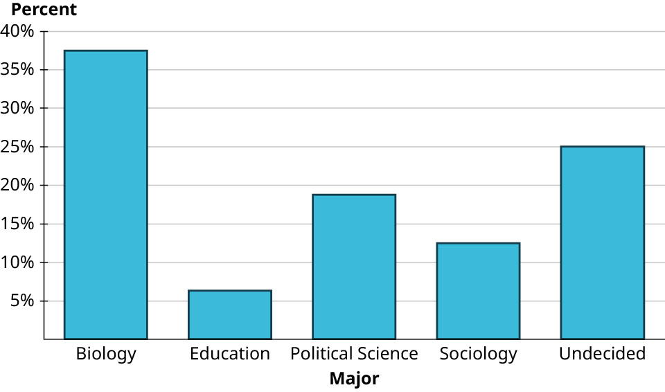
| Major | Frequency | Proportion |
|---|---|---|
| Biology | 6 | 37.5% |
| Education | 1 | 6.3% |
| Political Science | 3 | 18.8% |
| Sociology | 2 | 12.5% |
| Undecided | 4 | 25% |

| 4 | 7 |
| 5 | 9 7 4 |
| 6 | 9 8 7 |
| 7 | 8 7 5 2 2 1 0 |
| 8 | 9 6 5 4 4 1 |
| 9 | 7 7 6 3 3 1 |
| 10 | 7 6 3 1 |
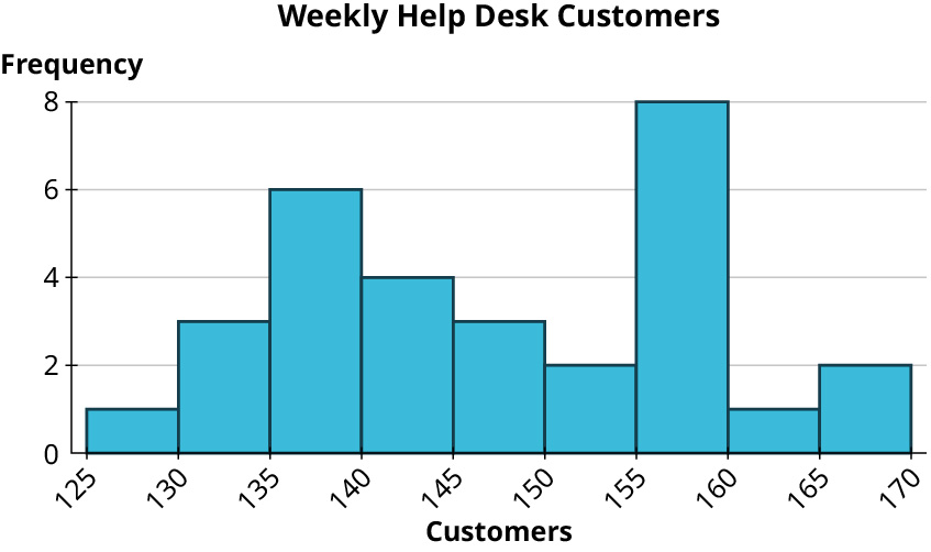
Answers may vary based on bin choices. Here’s the result for bins of width 2,500:

The data are strongly right-skewed.

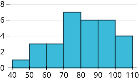
Top ten teams by wins:


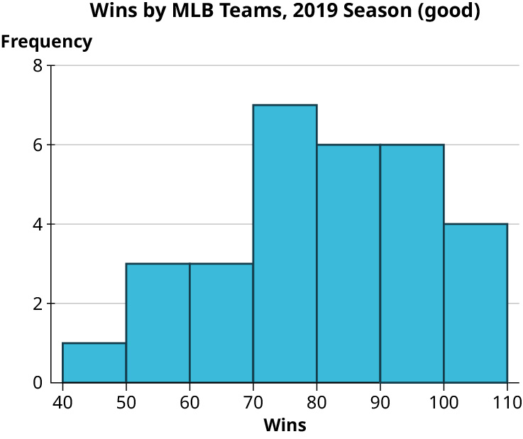

2
Median: 82.5
Mean: 80.967 (rounded to three decimal places)
\(s = \sqrt {752.5} \approx 27.432\)
The red (leftmost) distribution has mean 11, the blue (middle) has mean 13, and the yellow (rightmost) has mean 14.
65 and 75
26 and 54
110 and 290
47.5%
15.85%
81.5%
\(−1.8\)
\(1.6\)
\(−0.6\)
30
6
80th
9th
97th
3.9
6.3
2.9
Using NORM.INV: 1092.8
Using PERCENTILE: 1085
- No curved pattern
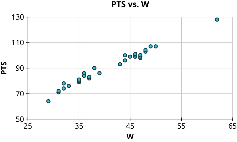
- Strong negative relationship, \(r \approx - 0.9\)
- Curved pattern
- No curved pattern
- No apparent relationship, \(r \approx 0\)
- No curved pattern
- Weak positive relationship, \(r \approx 0.6\)
- \(r = - 0.91\)
- Not appropriate
- \(r = - 0.01\)
- \(r = 0.62\)
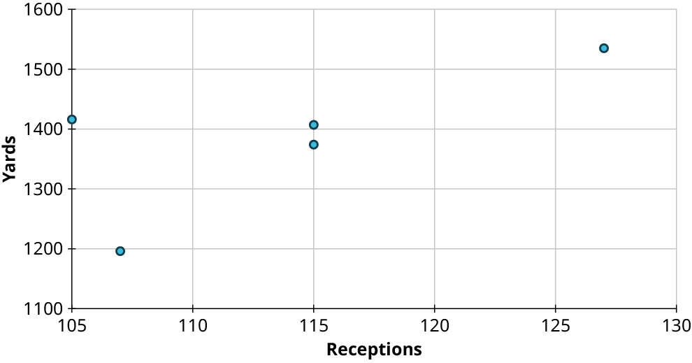
\(y = 1.8x + 16.9\)
\(y = 0.174x + 14.5\)
26.68
Predicted: 28; actual: 18. The Phillies were caught around 10 fewer times than expected.
Every 10 additional steal attempts will result in getting caught about 1.7 times on average.
Check Your Understanding
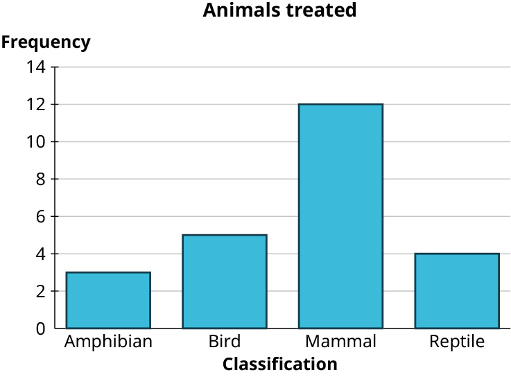
| Genre | Frequency |
|---|---|
| Cooking | 1 |
| Non-fiction | 3 |
| Romance | 4 |
| Thriller | 3 |
| True Crime | 3 |
| Young Adult | 6 |
| Number of classes | Frequency |
|---|---|
| 1 | 1 |
| 2 | 3 |
| 3 | 16 |
| 4 | 8 |
| 5 | 4 |
| Range of Cell Phone Subscriptions Per Hundred People | Frequency |
|---|---|
| 0.0 – 24.9 | 1 |
| 25.0 – 49.9 | 3 |
| 50.0 – 74.9 | 1 |
| 75.0 – 99.9 | 6 |
| 100.0 – 124.9 | 7 |
| 125.0 – 149.9 | 3 |
| 150.0 – 174.9 | 3 |
| 175.0 – 199.9 | 1 |
(Note: Answers may vary based on choices made about bins.)
| 12 | 7 |
| 13 | 0 2 3 6 6 7 8 9 9 |
| 14 | 1 2 3 3 6 8 8 |
| 15 | 3 3 5 6 6 6 7 7 8 8 |
| 16 | 4 7 8 |


Mode: 112
Median: 113
Mean: 112.64
156
147
147.2
Mode: not useful; every value appears only once
Median: 0.322
Mean: 0.3612
Mode: not useful; every value appears only once
Median: $42,952
Mean: $42924.78
Median: $11,207
Mean: $15,476.79
23.2
1300 on the SAT
PERCENTILE gives 20.86; NORM.INV gives 21.11.
PERCENTILE gives 11.82; NORM.INV gives 11.68.
PERCENTRANK gives 92.6th; NORM.DIST gives 91.9th.
PERCENTRANK gives 77th; NORM.DIST gives 79.2nd.
- Yes
- No
- Weak positive relationship; \(r \approx 0.5\)
0.96
$7,475
Less than expected by $1,495.68
For every $1,000 increase in out-of-state tuition, we expect average monthly salary to increase by $161.