2.4: Picturing Data with Graphics

Last updated
Save as PDF

Page ID: 148716

$ \newcommand{\vecs}[1]{\overset { \scriptstyle \rightharpoonup} {\mathbf{#1}} } $

$ \newcommand{\vecd}[1]{\overset{-\!-\!\rightharpoonup}{\vphantom{a}\smash {#1}}} $

$ \newcommand{\id}{\mathrm{id}}$ $ \newcommand{\Span}{\mathrm{span}}$

( \newcommand{\kernel}{\mathrm{null}\,}\) $ \newcommand{\range}{\mathrm{range}\,}$

$ \newcommand{\RealPart}{\mathrm{Re}}$ $ \newcommand{\ImaginaryPart}{\mathrm{Im}}$

$ \newcommand{\Argument}{\mathrm{Arg}}$ $ \newcommand{\norm}[1]{\| #1 \|}$

$ \newcommand{\inner}[2]{\langle #1, #2 \rangle}$

$ \newcommand{\Span}{\mathrm{span}}$

$ \newcommand{\id}{\mathrm{id}}$

$ \newcommand{\Span}{\mathrm{span}}$

$ \newcommand{\kernel}{\mathrm{null}\,}$

$ \newcommand{\range}{\mathrm{range}\,}$

$ \newcommand{\RealPart}{\mathrm{Re}}$

$ \newcommand{\ImaginaryPart}{\mathrm{Im}}$

$ \newcommand{\Argument}{\mathrm{Arg}}$

$ \newcommand{\norm}[1]{\| #1 \|}$

$ \newcommand{\inner}[2]{\langle #1, #2 \rangle}$

$ \newcommand{\Span}{\mathrm{span}}$ $ \newcommand{\AA}{\unicode[.8,0]{x212B}}$

$ \newcommand{\vectorA}[1]{\vec{#1}} % arrow$

$ \newcommand{\vectorAt}[1]{\vec{\text{#1}}} % arrow$

$ \newcommand{\vectorB}[1]{\overset { \scriptstyle \rightharpoonup} {\mathbf{#1}} } $

$ \newcommand{\vectorC}[1]{\textbf{#1}} $

$ \newcommand{\vectorD}[1]{\overrightarrow{#1}} $

$ \newcommand{\vectorDt}[1]{\overrightarrow{\text{#1}}} $

$ \newcommand{\vectE}[1]{\overset{-\!-\!\rightharpoonup}{\vphantom{a}\smash{\mathbf {#1}}}} $

$ \newcommand{\vecs}[1]{\overset { \scriptstyle \rightharpoonup} {\mathbf{#1}} } $

$ \newcommand{\vecd}[1]{\overset{-\!-\!\rightharpoonup}{\vphantom{a}\smash {#1}}} $

$\newcommand{\avec}{\mathbf a}$ $\newcommand{\bvec}{\mathbf b}$ $\newcommand{\cvec}{\mathbf c}$ $\newcommand{\dvec}{\mathbf d}$ $\newcommand{\dtil}{\widetilde{\mathbf d}}$ $\newcommand{\evec}{\mathbf e}$ $\newcommand{\fvec}{\mathbf f}$ $\newcommand{\nvec}{\mathbf n}$ $\newcommand{\pvec}{\mathbf p}$ $\newcommand{\qvec}{\mathbf q}$ $\newcommand{\svec}{\mathbf s}$ $\newcommand{\tvec}{\mathbf t}$ $\newcommand{\uvec}{\mathbf u}$ $\newcommand{\vvec}{\mathbf v}$ $\newcommand{\wvec}{\mathbf w}$ $\newcommand{\xvec}{\mathbf x}$ $\newcommand{\yvec}{\mathbf y}$ $\newcommand{\zvec}{\mathbf z}$ $\newcommand{\rvec}{\mathbf r}$ $\newcommand{\mvec}{\mathbf m}$ $\newcommand{\zerovec}{\mathbf 0}$ $\newcommand{\onevec}{\mathbf 1}$ $\newcommand{\real}{\mathbb R}$ $\newcommand{\twovec}[2]{\left[\begin{array}{r}#1 \\ #2 \end{array}\right]}$ $\newcommand{\ctwovec}[2]{\left[\begin{array}{c}#1 \\ #2 \end{array}\right]}$ $\newcommand{\threevec}[3]{\left[\begin{array}{r}#1 \\ #2 \\ #3 \end{array}\right]}$ $\newcommand{\cthreevec}[3]{\left[\begin{array}{c}#1 \\ #2 \\ #3 \end{array}\right]}$ $\newcommand{\fourvec}[4]{\left[\begin{array}{r}#1 \\ #2 \\ #3 \\ #4 \end{array}\right]}$ $\newcommand{\cfourvec}[4]{\left[\begin{array}{c}#1 \\ #2 \\ #3 \\ #4 \end{array}\right]}$ $\newcommand{\fivevec}[5]{\left[\begin{array}{r}#1 \\ #2 \\ #3 \\ #4 \\ #5 \\ \end{array}\right]}$ $\newcommand{\cfivevec}[5]{\left[\begin{array}{c}#1 \\ #2 \\ #3 \\ #4 \\ #5 \\ \end{array}\right]}$ $\newcommand{\mattwo}[4]{\left[\begin{array}{rr}#1 \amp #2 \\ #3 \amp #4 \\ \end{array}\right]}$ $\newcommand{\laspan}[1]{\text{Span}\{#1\}}$ $\newcommand{\bcal}{\cal B}$ $\newcommand{\ccal}{\cal C}$ $\newcommand{\scal}{\cal S}$ $\newcommand{\wcal}{\cal W}$ $\newcommand{\ecal}{\cal E}$ $\newcommand{\coords}[2]{\left\{#1\right\}_{#2}}$ $\newcommand{\gray}[1]{\color{gray}{#1}}$ $\newcommand{\lgray}[1]{\color{lightgray}{#1}}$ $\newcommand{\rank}{\operatorname{rank}}$ $\newcommand{\row}{\text{Row}}$ $\newcommand{\col}{\text{Col}}$ $\renewcommand{\row}{\text{Row}}$ $\newcommand{\nul}{\text{Nul}}$ $\newcommand{\var}{\text{Var}}$ $\newcommand{\corr}{\text{corr}}$ $\newcommand{\len}[1]{\left|#1\right|}$ $\newcommand{\bbar}{\overline{\bvec}}$ $\newcommand{\bhat}{\widehat{\bvec}}$ $\newcommand{\bperp}{\bvec^\perp}$ $\newcommand{\xhat}{\widehat{\xvec}}$ $\newcommand{\vhat}{\widehat{\vvec}}$ $\newcommand{\uhat}{\widehat{\uvec}}$ $\newcommand{\what}{\widehat{\wvec}}$ $\newcommand{\Sighat}{\widehat{\Sigma}}$ $\newcommand{\lt}{<}$ $\newcommand{\gt}{>}$ $\newcommand{\amp}{&}$ $\definecolor{fillinmathshade}{gray}{0.9}$

INTRODUCTION

You saw the graph below in Preparation 2.4:

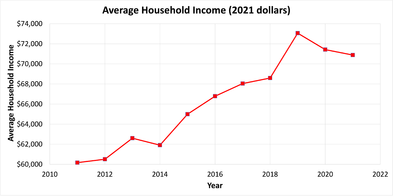
Based on the graph, discuss the following questions in your group:

How much did the Average Household Income increase from 2011 to 2019?
How much did the Average Household Income decrease from 2019 to 2021?

SPECIFIC OBJECTIVES

By the end of this collaboration, you should understand that

the scale on graphs can change the perception of the information they represent.
to fully understand a pie chart, the reference value must be known.

By the end of this collaboration, you should be able to

calculate relative change from a line graph.
estimate the absolute size of the portions of a pie chart given its reference value.
use data displayed on two graphs to estimate a third quantity.

PROBLEM SITUATION 1: READING LINE GRAPHS

Compare Graph 1 (from Preparation 2.4) and Graph 2 below.

Graph 1

Graph 2

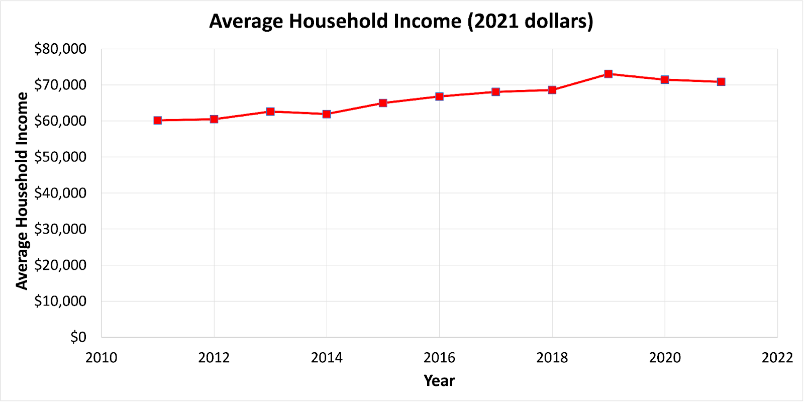
(1) What do you notice about the two graphs?

(2) Based on these two graphs, would it be fair to say that the average household income was significantly higher in 2021 than it was in 2011?

PROBLEM SITUATION 2: READING BAR GRAPHS

In Preparation 2.4, you were given two pairs of statements about Jeff’s housing expenditures. The statements are below for reference. You were asked to consider how both pairs of statements could be true. You were also asked to determine when Jeff spent more on housing. Your class will now discuss how understanding the answers to these questions can help you understand the gross domestic product (GDP) of a country. The gross domestic product is the value of all goods that are produced in a country in a certain time period, typically one year.

Pair 1

Pair 2

In 2000, Jeff spent $900 per month on housing.

In 2020, Jeff spent $1,800 per month on housing.

In 2000, Jeff spent 20% of his income on housing.

In 2020, Jeff spent 10% of his income on housing.

(3) Share your ideas from Preparation 2.4 with your group. Record two examples below.

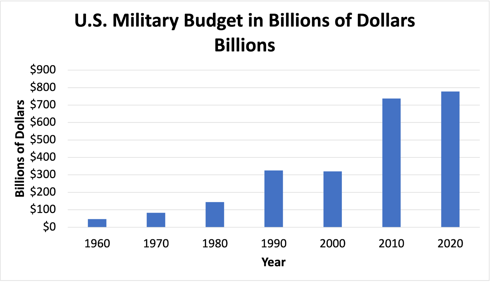
(4) Think about the statement, “The 2020 military budget is way out of hand and has never been higher.” You will use Graphs 3 and 4 to evaluate the statement.¹²

Graph 3

Vertical bar graph showing the US National Debt Trillions of Dollars from 1960 to 2020. Y-axis represents the amount in billions of dollars, ranging from 0 to 900. X-axis represents the years, ranging from 1960 to 2050. 1960 = just over 0 1970 = in between 0 and 100 1980 = in between 100 and 200 1990 = just over 300 2000 = about 300 2010 = in between 700 and 800 2020 = just under 800.

Graph 4

Vertical bar graph showing the US National Debt as a percent of GDP from 1960 to 2020. Y-axis represents the percent of GDP, ranging from 0 to 10. X-axis represents the years, ranging from 1960 to 2020. 1960 = about 9 1970 = about 8 1980 = about 5 1990 = about 6 2000 = about 3 2010 = about 5 2020 = about 4

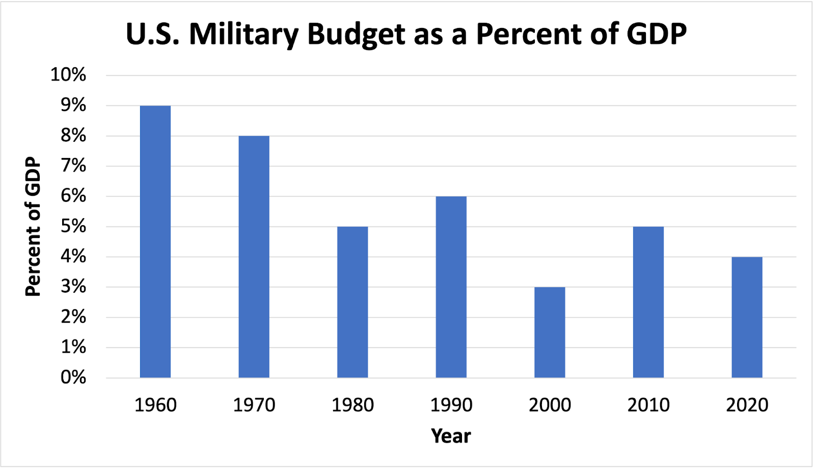
(4) Is the statement true? Based on what information?

PROBLEM SITUATION 3: READING PIE (CIRCLE) CHARTS

Refer to the graphs below,¹³^,14 to answer Questions 5 and 6. This pair of graphs cannot be used to predict that the number of non-Hispanics in the United States is expected to decline between 2020 and 2060.

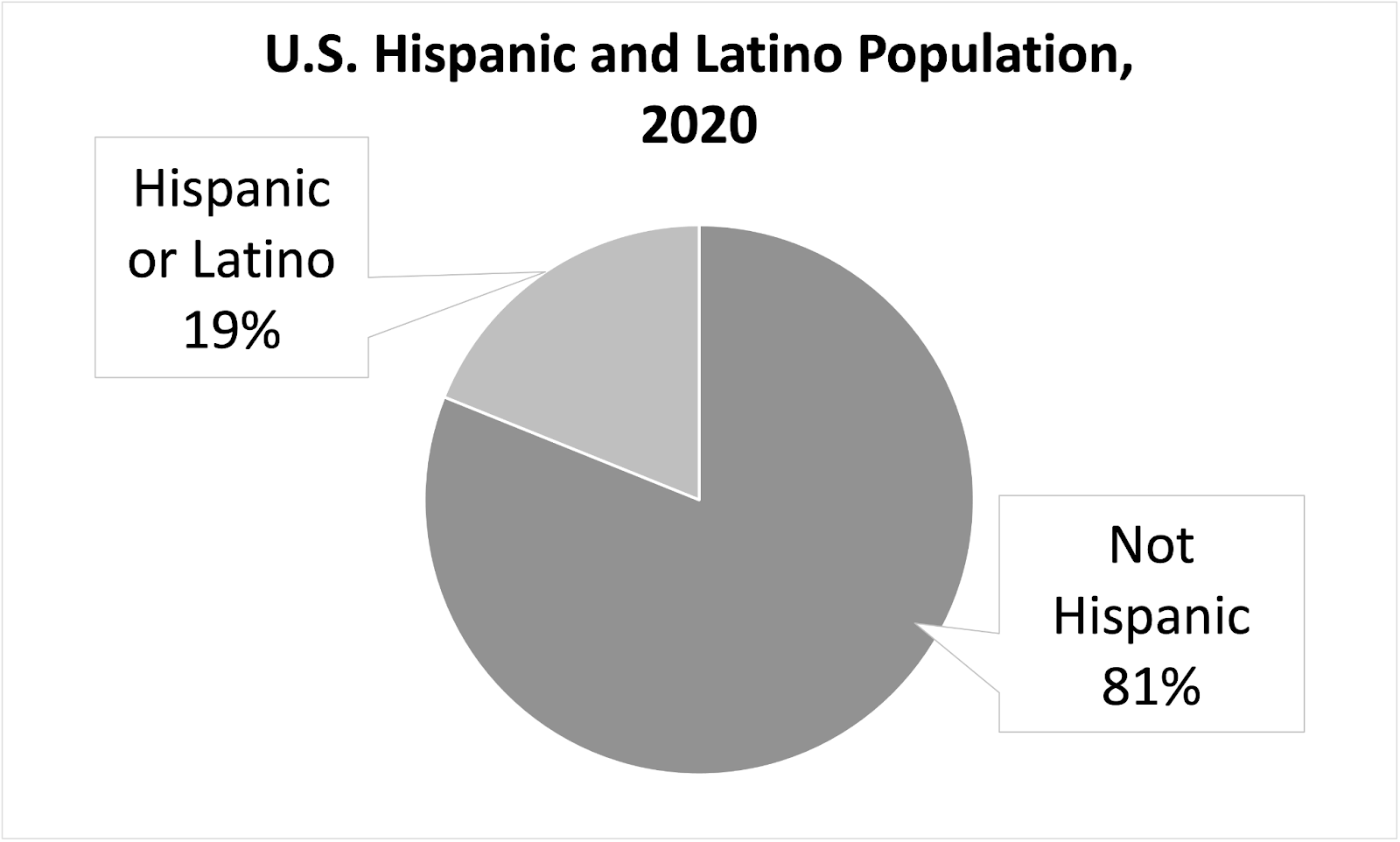
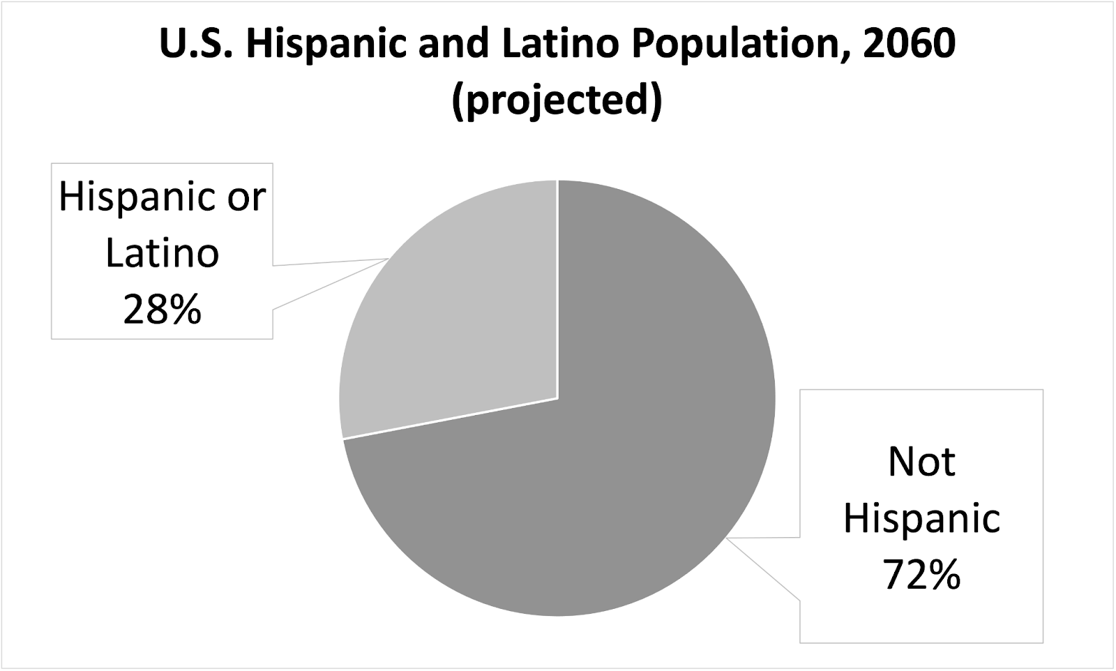
Circle graph showing the U.S. Hispanic Population for 2020. Hispanic = 19% Not Hispanic = 81%

Circle graph showing the Projected U.S. Hispanic Population for 2060. Hispanic = 28% Not Hispanic = 72%

(5) The U.S. population in 2020 was around 330,000,000. In 2060, the U.S. population is expected to be around 404,000,000. Estimate the number of Hispanic and non-Hispanic Americans at each time.

(6) Does your work in Question 5 confirm or contradict the notion that this pair of graphs cannot be used to predict that the number of non-Hispanics in the United States is expected to decline between 2020 and 2060? Explain.

FURTHER APPLICATIONS

(7) Write two different statements that compare the U.S. Hispanic population in 2020 to the projected U.S. Hispanic population in 2060.

Write your two statements here:

MAKING CONNECTIONS

Record the important mathematical ideas from the discussion.

___________________________________________

¹² https://www.macrotrends.net/countries/USA/united-states/military-spending-defense-budget

¹³ https://www.census.gov/quickfacts/fact/table/US/PST045221

¹⁴ https://www.census.gov/content/dam/Census/library/publications/2020/demo/p25-1144.pdf

Search

Text Color

Text Size

Margin Size

Font Type