2.4.1: Preparation 2.4

Last updated
Save as PDF

Page ID: 148717

$ \newcommand{\vecs}[1]{\overset { \scriptstyle \rightharpoonup} {\mathbf{#1}} } $

$ \newcommand{\vecd}[1]{\overset{-\!-\!\rightharpoonup}{\vphantom{a}\smash {#1}}} $

$ \newcommand{\id}{\mathrm{id}}$ $ \newcommand{\Span}{\mathrm{span}}$

( \newcommand{\kernel}{\mathrm{null}\,}\) $ \newcommand{\range}{\mathrm{range}\,}$

$ \newcommand{\RealPart}{\mathrm{Re}}$ $ \newcommand{\ImaginaryPart}{\mathrm{Im}}$

$ \newcommand{\Argument}{\mathrm{Arg}}$ $ \newcommand{\norm}[1]{\| #1 \|}$

$ \newcommand{\inner}[2]{\langle #1, #2 \rangle}$

$ \newcommand{\Span}{\mathrm{span}}$

$ \newcommand{\id}{\mathrm{id}}$

$ \newcommand{\Span}{\mathrm{span}}$

$ \newcommand{\kernel}{\mathrm{null}\,}$

$ \newcommand{\range}{\mathrm{range}\,}$

$ \newcommand{\RealPart}{\mathrm{Re}}$

$ \newcommand{\ImaginaryPart}{\mathrm{Im}}$

$ \newcommand{\Argument}{\mathrm{Arg}}$

$ \newcommand{\norm}[1]{\| #1 \|}$

$ \newcommand{\inner}[2]{\langle #1, #2 \rangle}$

$ \newcommand{\Span}{\mathrm{span}}$ $ \newcommand{\AA}{\unicode[.8,0]{x212B}}$

$ \newcommand{\vectorA}[1]{\vec{#1}} % arrow$

$ \newcommand{\vectorAt}[1]{\vec{\text{#1}}} % arrow$

$ \newcommand{\vectorB}[1]{\overset { \scriptstyle \rightharpoonup} {\mathbf{#1}} } $

$ \newcommand{\vectorC}[1]{\textbf{#1}} $

$ \newcommand{\vectorD}[1]{\overrightarrow{#1}} $

$ \newcommand{\vectorDt}[1]{\overrightarrow{\text{#1}}} $

$ \newcommand{\vectE}[1]{\overset{-\!-\!\rightharpoonup}{\vphantom{a}\smash{\mathbf {#1}}}} $

$ \newcommand{\vecs}[1]{\overset { \scriptstyle \rightharpoonup} {\mathbf{#1}} } $

$ \newcommand{\vecd}[1]{\overset{-\!-\!\rightharpoonup}{\vphantom{a}\smash {#1}}} $

$\newcommand{\avec}{\mathbf a}$ $\newcommand{\bvec}{\mathbf b}$ $\newcommand{\cvec}{\mathbf c}$ $\newcommand{\dvec}{\mathbf d}$ $\newcommand{\dtil}{\widetilde{\mathbf d}}$ $\newcommand{\evec}{\mathbf e}$ $\newcommand{\fvec}{\mathbf f}$ $\newcommand{\nvec}{\mathbf n}$ $\newcommand{\pvec}{\mathbf p}$ $\newcommand{\qvec}{\mathbf q}$ $\newcommand{\svec}{\mathbf s}$ $\newcommand{\tvec}{\mathbf t}$ $\newcommand{\uvec}{\mathbf u}$ $\newcommand{\vvec}{\mathbf v}$ $\newcommand{\wvec}{\mathbf w}$ $\newcommand{\xvec}{\mathbf x}$ $\newcommand{\yvec}{\mathbf y}$ $\newcommand{\zvec}{\mathbf z}$ $\newcommand{\rvec}{\mathbf r}$ $\newcommand{\mvec}{\mathbf m}$ $\newcommand{\zerovec}{\mathbf 0}$ $\newcommand{\onevec}{\mathbf 1}$ $\newcommand{\real}{\mathbb R}$ $\newcommand{\twovec}[2]{\left[\begin{array}{r}#1 \\ #2 \end{array}\right]}$ $\newcommand{\ctwovec}[2]{\left[\begin{array}{c}#1 \\ #2 \end{array}\right]}$ $\newcommand{\threevec}[3]{\left[\begin{array}{r}#1 \\ #2 \\ #3 \end{array}\right]}$ $\newcommand{\cthreevec}[3]{\left[\begin{array}{c}#1 \\ #2 \\ #3 \end{array}\right]}$ $\newcommand{\fourvec}[4]{\left[\begin{array}{r}#1 \\ #2 \\ #3 \\ #4 \end{array}\right]}$ $\newcommand{\cfourvec}[4]{\left[\begin{array}{c}#1 \\ #2 \\ #3 \\ #4 \end{array}\right]}$ $\newcommand{\fivevec}[5]{\left[\begin{array}{r}#1 \\ #2 \\ #3 \\ #4 \\ #5 \\ \end{array}\right]}$ $\newcommand{\cfivevec}[5]{\left[\begin{array}{c}#1 \\ #2 \\ #3 \\ #4 \\ #5 \\ \end{array}\right]}$ $\newcommand{\mattwo}[4]{\left[\begin{array}{rr}#1 \amp #2 \\ #3 \amp #4 \\ \end{array}\right]}$ $\newcommand{\laspan}[1]{\text{Span}\{#1\}}$ $\newcommand{\bcal}{\cal B}$ $\newcommand{\ccal}{\cal C}$ $\newcommand{\scal}{\cal S}$ $\newcommand{\wcal}{\cal W}$ $\newcommand{\ecal}{\cal E}$ $\newcommand{\coords}[2]{\left\{#1\right\}_{#2}}$ $\newcommand{\gray}[1]{\color{gray}{#1}}$ $\newcommand{\lgray}[1]{\color{lightgray}{#1}}$ $\newcommand{\rank}{\operatorname{rank}}$ $\newcommand{\row}{\text{Row}}$ $\newcommand{\col}{\text{Col}}$ $\renewcommand{\row}{\text{Row}}$ $\newcommand{\nul}{\text{Nul}}$ $\newcommand{\var}{\text{Var}}$ $\newcommand{\corr}{\text{corr}}$ $\newcommand{\len}[1]{\left|#1\right|}$ $\newcommand{\bbar}{\overline{\bvec}}$ $\newcommand{\bhat}{\widehat{\bvec}}$ $\newcommand{\bperp}{\bvec^\perp}$ $\newcommand{\xhat}{\widehat{\xvec}}$ $\newcommand{\vhat}{\widehat{\vvec}}$ $\newcommand{\uhat}{\widehat{\uvec}}$ $\newcommand{\what}{\widehat{\wvec}}$ $\newcommand{\Sighat}{\widehat{\Sigma}}$ $\newcommand{\lt}{<}$ $\newcommand{\gt}{>}$ $\newcommand{\amp}{&}$ $\definecolor{fillinmathshade}{gray}{0.9}$

Data are increasingly presented in a variety of forms intended to interest you and invite you to think about the importance of the data and how they might affect your lives. The following are some of the types of common displays:

Pie charts
Scatterplots
Histograms and bar graphs
Line graphs
Tables
Pictographs

What questions should you ask yourself when you study a visual display of information?

What is the title of the chart or graph?
What question is the data supposed to answer? (For example: How many males versus females exercise daily?)
How are the columns and rows labeled? How are the vertical and horizontal axes labeled?
Select one number or data point and ask, “What does this mean?”

Use the following chart to help you understand what some basic types of visual displays of information tell you and what questions they usually answer.

This looks like a …	This visual display is usually used to …	For example, it can be used to show …
pie chart	show the relationships between different parts compared to a whole.	how time is used in a 24-hour cycle. how money is distributed. how something is divided up.
line graph	show trends over time. compare trends of two different items or measurements.	what is increasing. what is decreasing. how the cost of gas has increased in the last 10 years. which of these foods (milk, steak, cookies, eggs) has risen most rapidly in price compared to the others.
histogram or bar graph	compare data in different categories. show changes over time.	how a population is broken up into different age categories. how college tuition rates are changing over time.
table	organize data to make specific values easy to read. break data up into overlapping categories.	the inflation rates over a period of years. how a population is broken into males and females of different age categories.

You will use the following information and your responses to Questions 9 - 11 in your next collaboration. Be sure to take notes.

(1) Use Graph 1 to answer the following questions.¹¹ (Note: The vertical axis starts at $60,000 instead of $0.)

Graph 1

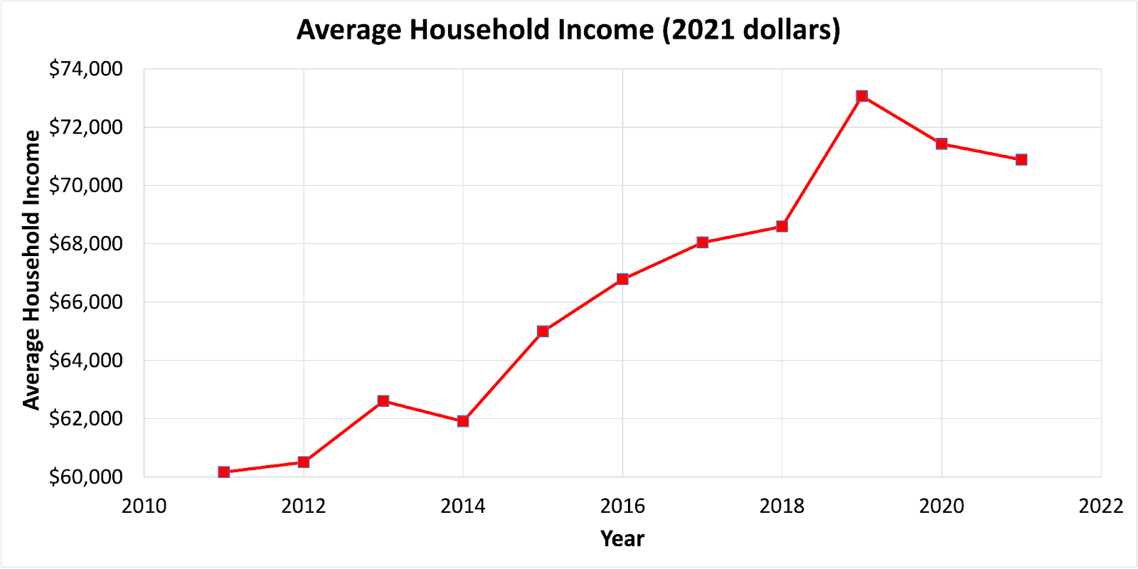
(a) Select the best phrase to complete this sentence: The numbers on the horizontal axis (the line across the bottom of the graph) represent…

(i) income from $2,010 to $2,022.

(ii) income from $2,010,000 to $2,022,000.

(iii) years from 2010 to 2022.

(iv) years and income.

(b) Select the best phrase to complete this sentence: The numbers on the vertical axis (the line along the left of the graph) represent…

(i) years from $60,000 to $74,000.

(ii) income for a household or family from $60,000 to $74,000.

(iii) income for one person from $60,000 to $74,000.

(iv) income in 2021 from $60,000 to $74,000.

(i) $66,000

(ii) $66,200

(iii) $66,800

(iv) $67,300

(d) A good estimate of the average household income in 2012 is

(i) $60,000

(ii) $60,500

(iii) $61,000

(iv) $61,400

(e) Use the estimates from (c) and (d) to calculate the relative change in the average household income from 2012 to 2016. Round to the nearest one percent. Indicate if the change is an increase or decrease.

(i) The relative change is…

(ii) The change is…

(2) Two pairs of statements about Jeff’s housing expenditures are given below. How can both pairs of statements be true? When did Jeff spend more on housing? Be prepared to discuss your answers in class.

Pair 1

Pair 2

In 2000, Jeff spent $900 per month on housing.

In 2020, Jeff spent $1,800 per month on housing.

In 2000, Jeff spent 20% of his income on housing.

In 2020, Jeff spent 10% of his income on housing.

After Preparation 2.4 (survey)

You should be able to do the following things for the next collaboration. Rate how confident you are on a scale of 1–5 (1 = not confident and 5 = very confident).

Before beginning Collaboration 2.4, you should understand the concepts and demonstrate the skills listed below.

Skill or Concept: I can …	Rating from 1 to 5
read a line graph.
read a bar graph.
read a pie graph.
calculate relative change.

Self-Regulated Learning: Reflect

Which problems from this lesson do you feel you understood well? Which ones might you find it beneficial to talk to your teacher or someone else about?

When planning to do this homework assignment, how accurately did you predict how long the assignment was going to take?

Name two strategies you used when solving problems in this assignment.

__________________________________________

¹¹ https://www.census.gov/data/tables/time-series/demo/income-poverty/historical-income-households.html

Search

Text Color

Text Size

Margin Size

Font Type