9.4: Measures of Variation
- Page ID
- 59979

Consider these three sets of quiz scores:
Section A: 5 5 5 5 5 5 5 5 5 5
Section B: 0 0 0 0 0 10 10 10 10 10
Section C: 4 4 4 5 5 5 5 6 6 6
All three of these sets of data have a mean of 5 and a median of 5, yet the sets of scores are clearly quite different. In section A, everyone had the same score; in section B, half the class got no points and the other half got a perfect score, assuming this was a 10-point quiz. Section C was not as consistent as section A, but not as widely varied as section B.
In addition to the mean and median, which are measures of the “typical” or “middle” value, we also need a measure of how “spread out” or varied each data set is.
There are several ways to measure this “spread” of the data. The first is the simplest and is called the range.
The range is the difference between the maximum value and the minimum value of the data set.
Using the quiz scores from above,
For section A, the range is \(0\) since both maximum and minimum are \(5\) and \(5 – 5 = 0\)
For section B, the range is \(10\) since \(10 – 0 = 10\)
For section C, the range is \(2\) since \(6 – 4 = 2\)
In the last example, the range seems to be revealing how spread out the data is. However, suppose we add a fourth section, Section D, with scores
0 5 5 5 5 5 5 5 5 10
This section also has a mean and median of 5. The range is 10, yet, this data set is quite different than Section B. To better illuminate the differences, we’ll have to turn to more sophisticated measures of variation.
The standard deviation is a measure of variation based on measuring the distance each data value deviates, or is different, from the mean. A few important characteristics:
- Standard deviation is always positive. Standard deviation will be zero if all the data values are equal, and will get larger as the data spreads out.
- Standard deviation has the same units as the original data.
- Standard deviation, like the mean, can be highly influenced by outliers.
Using the data from section D, we could compute for each data value the difference between the data value and the mean:
| Data Value | Deviation: Data Value - Mean |
| 0 | 0-5 = -5 |
| 5 | 5-5 = 0 |
| 5 | 5-5 = 0 |
| 5 | 5-5 = 0 |
| 5 | 5-5 = 0 |
| 5 | 5-5 = 0 |
| 5 | 5-5 = 0 |
| 5 | 5-5 = 0 |
| 5 | 5-5 = 0 |
| 10 | 10-5 = 0 |
We would like to get an idea of the “average” deviation from the mean, but if we find the average of the values in the second column the negative and positive values cancel each other out (this will always happen), so to prevent this we square every value in the second column:
| Data Value | Deviation: Data Value - Mean | (Deviation)2 |
| 0 | 0-5 = -5 | (-5)2 = 25 |
| 5 | 5-5 = 0 | 02 = 0 |
| 5 | 5-5 = 0 | 02 = 0 |
| 5 | 5-5 = 0 | 02 = 0 |
| 5 | 5-5 = 0 | 02 = 0 |
| 5 | 5-5 = 0 | 02 = 0 |
| 5 | 5-5 = 0 | 02 = 0 |
| 5 | 5-5 = 0 | 02 = 0 |
| 5 | 5-5 = 0 | 02 = 0 |
| 10 | 10-5 = 5 | (5)2 = 25 |
We then add the squared deviations up to get \(25 + 0 + 0 + 0 + 0 + 0 + 0 + 0 + 0 + 25 = 50\). Ordinarily, we would then divide by the number of scores, \(n\), (in this case, 10) to find the mean of the deviations. But we only do this if the data set represents a population; if the data set represents a sample (as it almost always does), we instead divide by \(n - 1\) (in this case, \(10 - 1 = 9\)) [4].
So, in our example, we would have \(\dfrac{50}{10} = 5\) if section D represents a population and \(\dfrac{50}{9} =\) about \(5.56\) if section D represents a sample. These values (\(5\) and \(5.56\)) are called, respectively, the population variance and the sample variance for section D.
Variance can be a useful statistical concept, but note that the units of variance in this instance would be points-squared since we squared all of the deviations. What are points-squared? Good question. We would rather deal with the units we started with (points in this case), so to convert back we take the square root and get:
\(\text{Population Standard Deviation } = \sqrt{\dfrac{50}{10}} = \sqrt{5} ≈ 2.2\)
\(\text{Sample Standard Deviation } = \sqrt{\dfrac{50}{9}} ≈ 2.4\)
What does this say about section D? We can say that the average score was 5 give or take 2.4. The “give or take” part is the prefix for standard deviation. In the last chapter, we discuss more about the relationship between the average and standard deviation. For now, we can interpret results as “the average is ________ give or take [standard deviation].”
If we are unsure whether the data set is a sample or a population, we will usually assume it is a sample, and we will round answers to one more decimal place than the original data, as we have done above.
- Find the deviation of each data from the mean. In other words, subtract the mean from the data value.
- Square each deviation.
- Add the squared deviations.
- Divide by \(n\), the number of data values, if the data represents a whole population; divide by \(n – 1\) if the data is from a sample. (This result is the sample variance.)
- Compute the square root of the result. (This result is the standard deviation.)
Computing the standard deviation for Section B above, we first calculate that the mean is 5. Using a table can help keep track of your computations for the standard deviation:
| Data Value | Deviation: Data Value - Mean | (Deviation)2 |
| 0 | 0-5 = -5 | (-5)2 = 25 |
| 0 | 0-5 = -5 | (-5)2 = 25 |
| 0 | 0-5 = -5 | (-5)2 = 25 |
| 0 | 0-5 = -5 | (-5)2 = 25 |
| 0 | 0-5 = -5 | (-5)2 = 25 |
| 10 | 10-5 = 5 | (5)2 = 25 |
| 10 | 10-5 = 5 | (5)2 = 25 |
| 10 | 10-5 = 5 | (5)2 = 25 |
| 10 | 10-5 = 5 | (5)2 = 25 |
| 10 | 10-5 = 5 | (5)2 = 25 |
Assuming this data represents a population, we will add the squared deviations, divide by 10, the number of data values, and compute the square root:
\(\sqrt{\dfrac{25 + 25 + 25 + 25 + 25 + 25 + 25 + 25 + 25 + 25}{10}} = \sqrt{\dfrac{250}{10}} = 5\)
Notice that the standard deviation of this data set is much larger than that of section D since the data in this set is more spread out. Thus, the average score was 5 give or take 5.
For comparison, the standard deviations of all four sections are
| Section A: 5 5 5 5 5 5 5 5 5 5 | Standard deviation: 0 |
| Section B: 0 0 0 0 0 10 10 10 10 10 | Standard deviation: 5 |
| Section C: 4 4 4 5 5 5 5 6 6 6 | Standard deviation: 0.8 |
| Section D: 0 5 5 5 5 5 5 5 5 10 | Standard deviation: 2.2 |
The price of a jar of peanut butter at 5 stores were: $3.29, $3.59, $3.79, $3.75, and $3.99. Find the standard deviation of the prices.
Where standard deviation is a measure of variation based on the mean, quartiles are based on the median.
Quartiles are values that divide the data in quarters.
The first quartile (Q1) is the value so that 25% of the data values are below it; the third quartile (Q3) is the value so that 75% of the data values are below it. You may have guessed that the second quartile is the same as the median, since the median is the value so that 50% of the data values are below it.
This divides the data into quarters; 25% of the data is between the minimum and Q1, 25% is between Q1 and the median, 25% is between the median and Q3, and 25% is between Q3 and the maximum value
While quartiles are not a 1-number summary of variation like standard deviation, the quartiles are used with the median, minimum, and maximum values to form a 5-number summary of the data.
The five-number summary takes this form
Minimum, Q1, Median, Q3, Maximum
To find the first quartile, we need to find the data value so that 25% of the data is below it. If \(n\) is the number of data values, we compute a locator by finding 25% of \(n\). If this locator is a decimal value, we round up and find the data value in that position. If the locator is a whole number, we find the mean of the data value in that position and the next data value. This is identical to the process we used to find the median, except we use 25% of the data values rather than half the data values as the locator.
- Begin by ordering the data from smallest to largest.
- Compute the locator: \(L = 0.25n\).
- If \(L\) is a decimal value:
- Round up to \(L+\)
- Use the data value in the \(L+^{\text{th}}\) position.
If \(L\) is a whole number:
- Find the mean of the data values in the \(L^{\text{th}}\) and \(L+1^{\text{th}}\) positions.
Use the same procedure as for Q1, but with locator: \(L = 0.75n\)
Let’s look at some examples. We can also calculate the 5-number summary in calculators, or some scientific software like Excel, Minitab, or R. However, in this course, we only get our feet wet with statistics, so we can calculate these values quickly by hand.
Suppose we have measured 9 females and their heights (in inches), sorted from smallest to largest are:
59 60 62 64 66 67 69 70 72
To find the first quartile we first compute the locator: 25% of 9 is \(L = 0.25(9) = 2.25\). Since this value is not a whole number, we round up to 3. The first quartile will be the third data value: 62 inches. We can say that 25% of females are shorter than 62 inches and the other 75% is taller than 62 inches.
To find the third quartile, we again compute the locator: 75% of 9 is \(0.75(9) = 6.75\). Since this value is not a whole number, we round up to 7. The third quartile will be the seventh data value: 69 inches. We can say that 75% of females are shorter than 69 inches and the other 25% is taller than 69 inches.
Suppose we had measured 8 females and their heights (in inches), sorted from smallest to largest are:
59 60 62 64 66 67 69 70
To find the first quartile we first compute the locator: 25% of 8 is \(L = 0.25(8) = 2\). Since this value is a whole number, we will find the mean of the 2nd and 3rd data values: \(\dfrac{(60+62)}{2} = 61\), so the first quartile is 61 inches. We can say that the 25% of females are shorter than 61 inches and the other 75% is taller than 61 inches.
The third quartile is computed similarly, using 75% instead of 25%. \(L = 0.75(8) = 6\). This is a whole number, so we will find the mean of the 6th and 7th data values: \(\dfrac{(67+69)}{2} = 68\), so Q3 is 68 inches. We can say that the 75% of females are shorter than 68 inches and the other 25% is taller than 68 inches.
Note, the median could be computed the same way, using 50% or a locator of \(L = 0.5n\)
The 5-number summary combines the first and third quartile with the minimum, median, and maximum values.
In the example with a sample of 9 females, the median is 66, the minimum is 59, and the maximum is 72. Hence, the 5-number summary is:
59, 62, 66, 69, 72.
In the example with a sample of 8 females, the median is 65, the minimum is 59, and the maximum is 70, so the 5-number summary is:
59, 61, 65, 68, 70.
Returning to our quiz score data. In each case, the first quartile locator is 0.25(10) = 2.5, so the first quartile will be the 3rd data value, and the third quartile will be the 8th data value. Creating the five-number summaries:
| Section and Data | 5-Number Summary |
| Section A: 5 5 5 5 5 5 5 5 5 5 | Standard deviation: 0 |
| Section B: 0 0 0 0 0 10 10 10 10 10 | Standard deviation: 5 |
| Section C: 4 4 4 5 5 5 5 6 6 6 | Standard deviation: 0.8 |
| Section D: 0 5 5 5 5 5 5 5 5 10 | Standard deviation: 2.2 |
Of course, with a relatively small data set, finding a five-number summary is a bit silly, since the summary contains almost as many values as the original data.
The total cost of textbooks for the term was collected from 36 students. Find the 5-number summary of this data.
$140 $160 $160 $165 $180 $220 $235 $240 $250 $260 $280 $285
$285 $285 $290 $300 $300 $305 $310 $310 $315 $315 $320 $320
$330 $340 $345 $350 $355 $360 $360 $380 $395 $420 $460 $460
Returning to the household income data from earlier, create the five-number summary.
| Income (thousands of dollars) | Frequency |
| $15 | 6 |
| $20 | 8 |
| $25 | 11 |
| $30 | 17 |
| $35 | 19 |
| $40 | 20 |
| $45 | 12 |
| $50 | 7 |
By adding the frequencies, we can see there are 100 data values represented in the table. In Example 9.3.7, we found the median was $35 thousand. We can see in the table that the minimum income is $15 thousand, and the maximum is $50 thousand.
To find Q1, we calculate the locator: \(L = 0.25(100) = 25\). This is a whole number, so Q1 will be the mean of the 25th and 26th data values.
Counting up in the data as we did before,
There are 6 data values of $15, so Values 1 to 6 are $15 thousand
The next 8 data values are $20, so Values 7 to \((6+8)=14\) are $20 thousand
The next 11 data values are $25, so Values 15 to \((14+11)=25\) are $25 thousand
The next 17 data values are $30, so Values 26 to \((25+17)=42\) are $30 thousand
The 25th data value is $25 thousand, and the 26th data value is $30 thousand, so Q1 will be the mean of these: \(\dfrac{(25 + 30)}{2} = $27.5\) thousand.
To find Q3, we calculate the locator: \(L = 0.75(100) = 75\). This is a whole number, so Q3 will be the mean of the 75th and 76th data values. Continuing our counting from earlier,
The next 19 data values are $35, so Values 43 to \((42+19)=61\) are $35 thousand
The next 20 data values are $40, so Values 61 to \((61+20)=81\) are $40 thousand
Both the 75th and 76th data values lie in this group, so Q3 will be $40 thousand.
Putting these values together into a five-number summary, we get: 15, 27.5, 35, 40, 50.
Note that the 5-number summary divides the data into four intervals, each of which will contain about 25% of the data. In the previous example, about 25% of households have income between $40 thousand and $50 thousand. For visualizing data, there is a graphical representation of a 5-number summary called a box plot, or box and whisker graph.
For visualizing data, there is a graphical representation of a 5-number summary called a box plot, or box and whisker graph.
A box plot is a graphical representation of a five-number summary.
To create a box plot, a number line is first drawn with equidistant tick marks. A box is drawn from the first quartile to the third quartile, and a line is drawn through the box at the median. “Whiskers” are extended out to the minimum and maximum values.
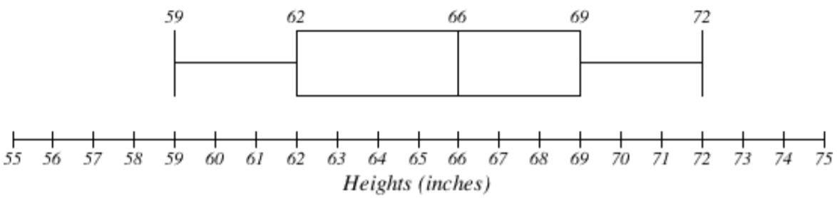
The box plot below is based on the 5-number summary from the sample of 9 female heights:
59, 62, 66, 69, 72
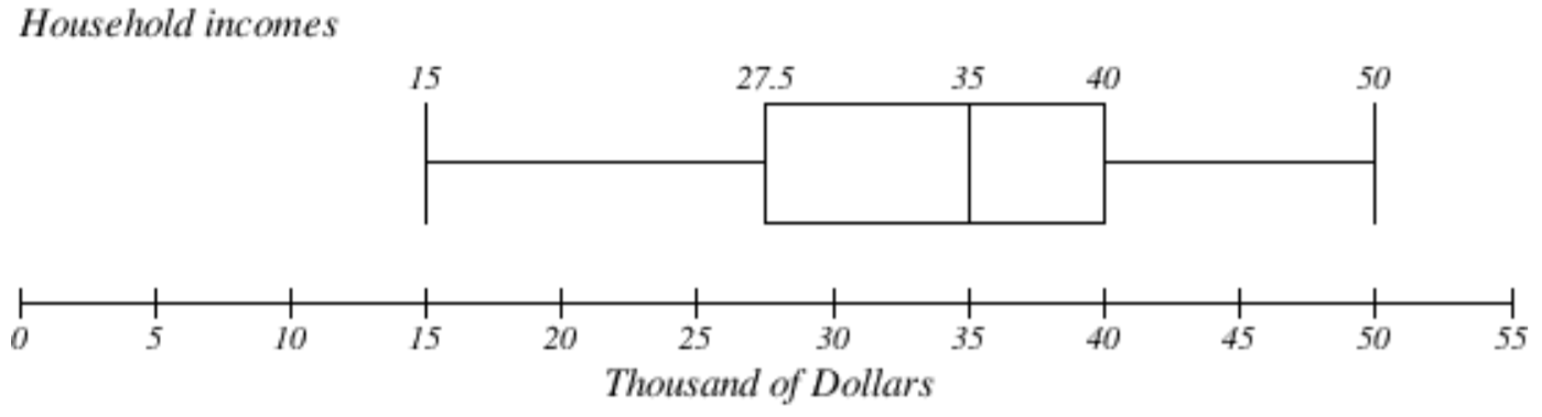
The box plot below is based on the 5-number summary from the sample of the household incomes:
15, 27.5, 35, 40, 50
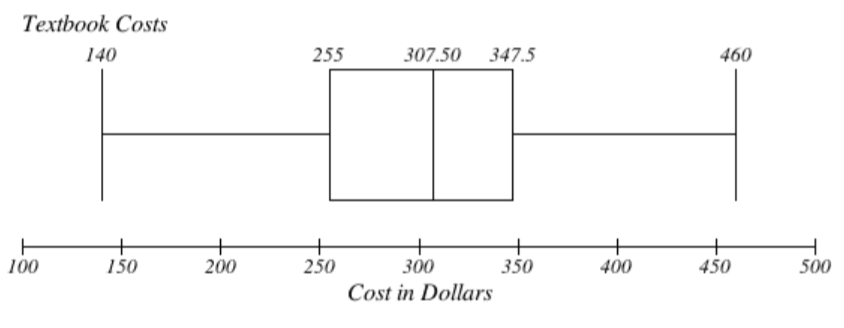
Create a boxplot based on the textbook price data from the last Try it Now.
Box plots are particularly useful for comparing data from two populations or samples. In fact, when we have two samples to compare, it is always preferred to use box plots.
The box plot of service times for two fast-food restaurants is shown below.
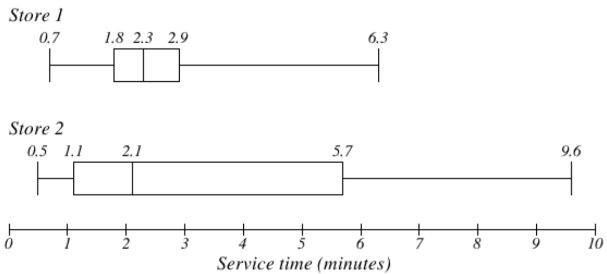
While store 2 had a slightly shorter median service time (2.1 minutes vs. 2.3 minutes), store 2 is less consistent, with a wider spread of the data.
At store 1, 75% of customers were served within 2.9 minutes, while at store 2, 75% of customers were served within 5.7 minutes.
Which store should you go to in a hurry? That depends upon your opinions about luck – 25% of customers at store 2 had to wait between 5.7 and 9.6 minutes.
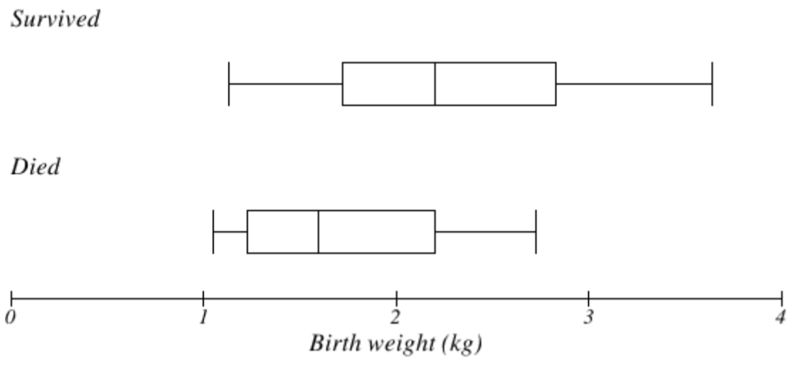
The boxplot below is based on the birth weights of infants with severe idiopathic respiratory distress syndrome (SIRDS) [5]. The boxplot is separated to show the birth weights of infants who survived and those that did not.
Comparing the two groups, the boxplot reveals that the birth weights of the infants that died appear to be, overall, smaller than the weights of infants that survived. In fact, we can see that the median birth weight of infants that survived is the same as the third quartile of the infants that died.
Similarly, we can see that the first quartile of the survivors is larger than the median weight of those that died, meaning that over 75% of the survivors had a birth weight larger than the median birth weight of those that died.
Looking at the maximum value for those that died and the third quartile of the survivors, we can see that over 25% of the survivors had birth weights higher than the heaviest infant that died.
The box plot gives us a quick, albeit informal, way to determine that birth weight is quite likely linked to survival of infants with SIRDS.
1.
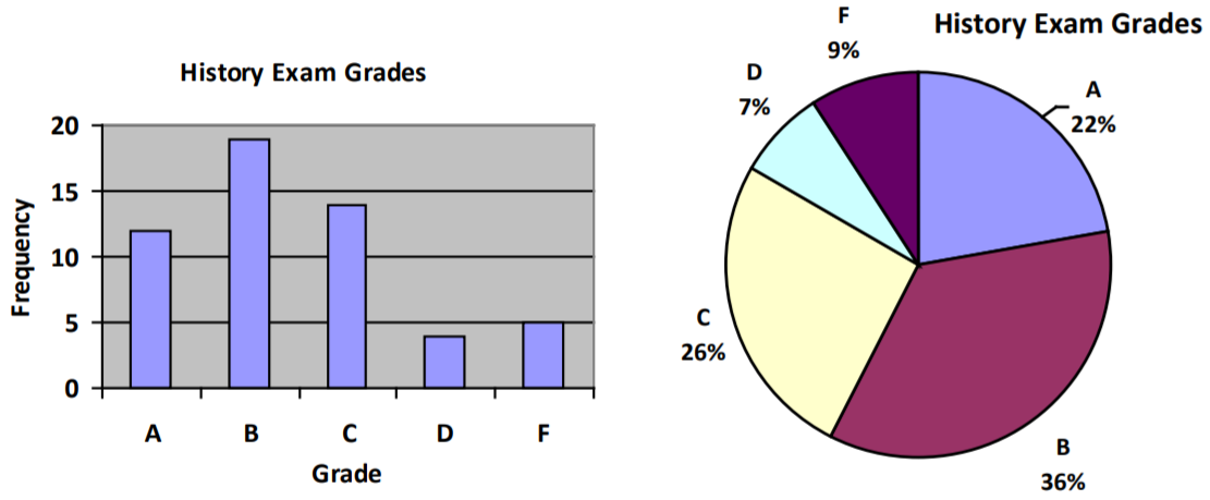
2. While the pie chart accurately depicts the relative size of the people agreeing with each candidate, the chart is confusing, since usually percents on a pie chart represent the percentage of the pie the slice represents.
3. Using a class intervals of size 55, we can group our data into six intervals:
| Cost interval | Frequency |
| $140-194 | 5 |
| $195-249 | 3 |
| $250-304 | 9 |
| $305-359 | 12 |
| $360-414 | 4 |
| $415-469 | 3 |
We can use the frequency distribution to generate the histogram.
4. Adding the prices and dividing by 5 we get the mean price: $3.682
5. First we put the data in order: $3.29, $3.59, $3.75, $3.79, $3.99. Since there are an odd number of data, the median will be the middle value, $3.75.
6. There are 23 ratings.
a. The mean is \(\dfrac{(1 \cdot 4) + (2 \cdot 8) + (3 \cdot 7) + (4 \cdot 3) + (5 \cdot 1)}{23} ≈ 2.5\)
b. There are 23 data values, so the median will be the 12th data value. Ratings of 1 are the first 4 values, while a rating of 2 are the next 8 values, so the 12th value will be a rating of 2. The median is 2.
c. The mode is the most frequent rating. The mode rating is 2.
7. Earlier we found the mean of the data was $3.682.
| Data Value | Deviation: Data Value - Mean | Deviation Squared |
| 3.29 | 3.29 – 3.682 = -0.391 | 0.153664 |
| 3.59 | 3.59 – 3.682 = -0.092 | 0.008464 |
| 3.79 | 3.79 – 3.682 = 0.108 | 0.011664 |
| 3.75 | 3.75 – 3.682 = 0.068 | 0.004624 |
| 3.99 | 3.99 – 3.682 = 0.308 | 0.094864 |
This data is from a sample, so we will add the squared deviations, divide by 4, the number of data values minus 1, and compute the square root:
\(\sqrt{\dfrac{0.153664 + 0.008464 + 0.011664 + 0.004624 + 0.094864}{4}} ≈ $0.261\)
Thus, the average price of peanut butter is $3.68 give or take $0.26.
8. The data is already in order, so we don’t need to sort it first. The minimum value is $140 and the maximum is $460.
There are 36 data values so \(n = 36\). \(\dfrac{n}{2} = 18\), which is a whole number, so the median is the mean of the 18th and 19th data values, $305 and $310. The median is $307.50.
To find the first quartile, we calculate the locator, \(L = 0.25(36) = 9\). Since this is a whole number, we know Q1 is the mean of the 9th and 10th data values, $250 and $260. Q1 = $255.
To find the third quartile, we calculate the locator, \(L = 0.75(36) = 27\). Since this is a whole number, we know Q3 is the mean of the 27th and 28th data values, $345 and $350. Q3 = $347.50.
The 5-number summary of this data is: $140, $255, $307.50, $347.50, $460
9. Boxplot of textbook costs: