2.6: Continuous Age-Structured Populations

We can derive a continuous-time model by considering the discrete model in the limit as the age span $\Delta a$ of an age class (also equal to the time between censuses) goes to zero. For $n>\omega,(2.5.3)$ can be rewritten as

$$u_{1, n}=\sum_{i=1}^{\omega} f_{i} u_{1, n-i} \nonumber$$

The first age class in the discrete model consists of females born between two consecutive censuses. The corresponding function in the continuous model is the female birth rate of the population as a whole, $B(t)$, satisfying

$$u_{1, n}=B\left(t_{n}\right) \Delta a \nonumber$$

If we assume that the $n$th census takes place at a time $t_{n}=n \Delta a$, we also have

$$\begin{aligned} u_{1, n-i} &=B\left(t_{n-i}\right) \Delta a \\[4pt] &=B\left(t_{n}-t_{i}\right) \Delta a \end{aligned} \nonumber$$

To determine the continuous analogue of the parameter $f_{i}=m_{i} l_{i}$, we define the agespecific survival function $l(a)$ to be the fraction of newborn females that survive to age $a$, and define the age-specific maternity function $m(a)$, multiplied by $\Delta a$, to be the average number of females born to a female between the ages of $a$ and $a+\Delta a$. With the definition of the age-specific net maternity function, $f(a)=m(a) l(a)$, and $a_{i}=i \Delta a$, we have

$$f_{i}=f\left(a_{i}\right) \Delta a \nonumber$$

With these new definitions, $(2.6.1)$ becomes

$$B\left(t_{n}\right) \Delta a=\sum_{i=1}^{\omega} f\left(a_{i}\right) B\left(t_{n}-t_{i}\right)(\Delta a)^{2} \nonumber$$

Canceling one factor of $\Delta a$, and using $t_{i}=a_{i}$, the right-hand side becomes a Riemann sum. Taking $t_{n}=t$ and assigning $f(a)=0$ when $a$ is greater than the maximum age of female fertility, the limit $\Delta a \rightarrow 0$ transforms $(2.6.1)$ to

$$B(t)=\int_{0}^{\infty} B(t-a) f(a) d a . \nonumber$$

Equation (2.6.5) states that the population-wide female birth rate at time $t$ has contributions from females of all ages, and that the contribution to this birth rate from females between the ages of $a$ and $a+d a$ is determined from the population-wide female birth rate at the earlier time $t-a$ times the fraction of females that survive to age $a$ times the number of female births to females between the ages of $a$ and $a+d a$. Equation $(2.6.5)$ is a linear homogeneous integral equation, valid for $t$ greater than the maximum age of female fertility. A more complete but inhomogeneous equation valid for smaller $t$ can also be derived.

Equation (2.6.5) can be solved by the ansatz $B(t)=e^{r t}$. Direct substitution yields

$$e^{r t}=\int_{0}^{\infty} f(a) e^{r(t-a)} d a \nonumber$$

which upon canceling $e^{r t}$ results in the continuous Euler-Lotka equation

$$\int_{0}^{\infty} f(a) e^{-r a} d a=1 \nonumber$$

Equation (2.6.7) is an integral equation for $r$ given the age-specific net maternity function $f(a)$. It is possible to prove that for $f(a)$ a continuous non-negative function, (2.6.7) has exactly one real root $r_{*}$, and that the population grows $\left(r_{*}>0\right)$ or decays $\left(r_{*}<0\right)$ asymptotically as $e^{r_{*} t}$. The population growth rate $r_{*}$ has been called the intrinsic rate of increase, the intrinsic growth rate, or the Malthusian parameter. Typically, (2.6.7) is solved numerically for $r$ using a root-finding algorithm such as Newton’s method.

After asymptotically attaining a stable age structure, the population grows like $e^{r_{*} t}$, and our previous discussion of the Malthusian growth model suggests that $r_{*}$ may be found from the constant per capita birth rate $b$ and death rate $d$. By determining expressions for $b$ and $d$, we will indeed show that $r_{*}=b-d$.

Figure 2.4: Caenorhabditis elegans, a nematode worm used by biologists as a simple animal model of a multicellular organism. (Photo by Amy Pasquinelli.)

and the difference between the per capita birth and death rates is calculated from

$$b(t)-d(t)=\frac{\int_{0}^{\infty} B(t-a)[f(a)-g(a)] d a}{\int_{0}^{\infty} B(t-a) l(a) d a} \nonumber$$

Asymptotically, a stable age structure is established and the population-wide birth rate grows as $B(t) \sim e^{r_{*} t}$. Substitution of this expression for $B(t)$ into $(2.6.13)$ and cancelation of $e^{r_{*} t}$ results in

$$\begin{aligned} b-d &=\frac{\int_{0}^{\infty}[f(a)-g(a)] e^{-r_{*} a} d a}{\int_{0}^{\infty} l(a) e^{-r_{*} a} d a} \\[4pt] &=\frac{1+\int_{0}^{\infty} l^{\prime}(a) e^{-r_{*} a} d a}{\int_{0}^{\infty} l(a) e^{-r_{*} a} d a} \end{aligned} \nonumber$$

where use has been made of $(2.6.7)$ and $(2.6.11)$. Simplifying the numerator using integration by parts,

$$\begin{aligned} \int_{0}^{\infty} l^{\prime}(a) e^{-r_{*} a} d a &=\left.l(a) e^{-r_{*} a}\right|_{0} ^{\infty}+r_{*} \int_{0}^{\infty} l(a) e^{-r_{*} a} d a \\[4pt] &=-1+r_{*} \int_{0}^{\infty} l(a) e^{-r_{*} a} d a \end{aligned} \nonumber$$

produces the desired result,

$$r_{*}=b-d \nonumber$$

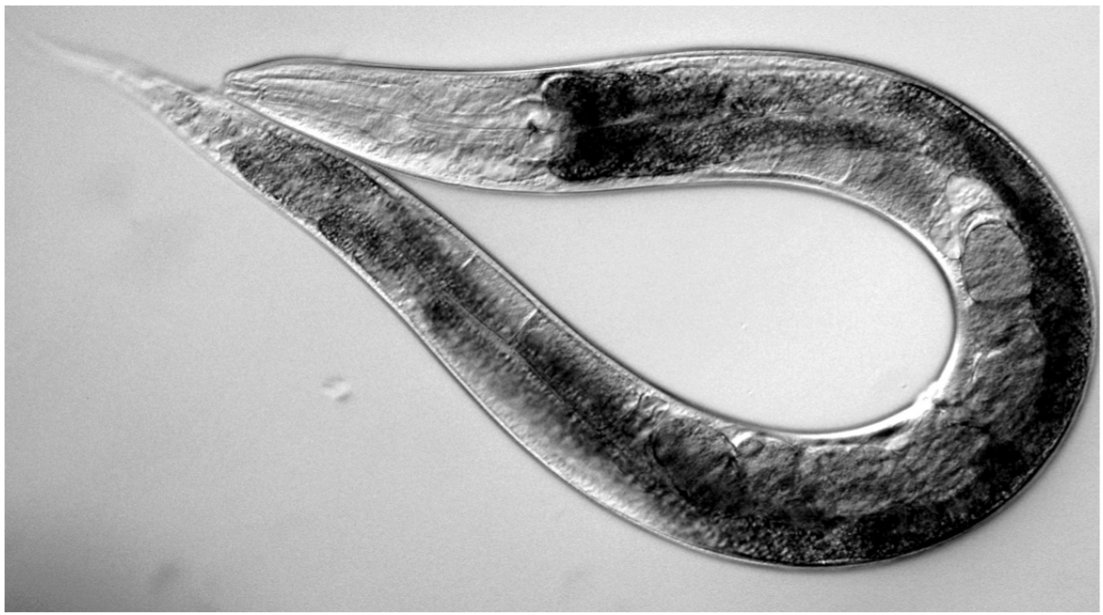
It is usually supposed that evolution by natural selection will result in populations with the largest value of the Malthusian parameter $r_{*}$, and that natural selection would favor those females that constitute such a population. We will exploit this idea in the next section to compute the brood size of the self-fertilizing hermaphroditic worm of the species Caenorhabditis elegans.