2.7: The Brood Size of a Hermaphroditic Worm

Caenorhabditis elegans, a soil-dwelling nematode worm about \(1 \mathrm{~mm}\) in length, is a widely studied model organism in biology. With a body made up of approximately

Figure 2.5: A simplified timeline of a hermaphrodite’s life.

1000 cells, it is one of the simplest multicellular organisms under study. Advances in understanding the development of this multicellular organism led to the awarding of the 2002 Nobel prize in Physiology or Medicine to the three C. elegans biologists Sydney Brenner, H. Robert Horvitz and John E. Sulston.

The worm C. elegans has two sexes: hermaphrodites, which are essentially females that can produce internal sperm and self-fertilize their own eggs, and males, which must mate with hermaphrodites to produce offspring. In laboratory cultures, males are rare and worms generally propagate by self-fertilization. Typically, a hermaphrodite lays about \(250-350\) self-fertilized eggs before becoming infertile. It is reasonable to assume that the forces of natural selection have shaped the lifehistory of C. elegans, and that the number of offspring produced by a selfing hermaphrodite must be in some sense optimal. Here, we show how an age-structured model applied to C. elegans yields theoretical insights into the brood size of a selfing hermaphrodite.

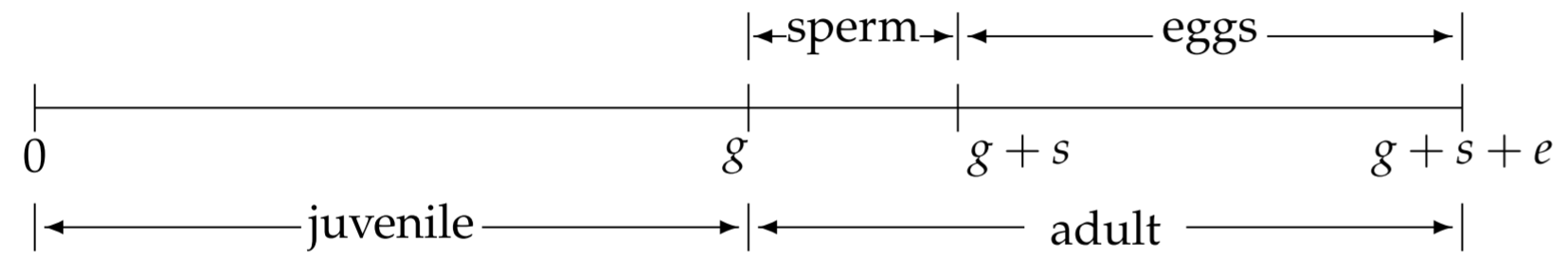
To develop a mathematical model for C. elegans, we need to know some details of its life history. As a first approximation (Barker, 1992), a simplified timeline of a hermaphrodite’s life is shown in Fig. 2.5. The fertilized egg is laid at time \(t=0\). During a juvenile growth period, the immature worm develops through four larval stages (L1-L4). Towards the end of L4 and for a short while after its final molt to adulthood, the hermaphrodite produces sperm, which is then stored for later use. Then the hermaphrodite produces eggs, self-fertilizes them using her internally stored sperm, and lays them. In the absence of males, egg production ceases after all the sperm are utilized. We assume that the juvenile growth period occurs during \(0<t<g\), spermatogenesis occurs during \(g<t<g+s\), and egg-production, selffertilization, and egg laying occurs during \(g+s<t<g+s+e\).

Here, we want to understand why hermaphrodites limit their sperm production. Biologists define males and females from the size and metabolic cost of their gametes: sperm are small and cheap and eggs are large and expensive. So on first look, it is puzzling why the total number of offspring produced by a hermaphrodite is limited by the number of sperm produced, rather than by the number of eggs. There must be a hidden cost to the hermaphrodite of producing additional sperm other than metabolic. To understand the basic biology, it is instructive to consider two limiting cases: (1) no sperm production; (2) infinite sperm production. In both cases, the hermaphrodite produces no offspring-in the first case because there are no sperm, and in the second case because there are no eggs. The number of sperm produced by a hermaphrodite before laying eggs is therefore a compromise; although more sperm means more offspring, more sperm also means delayed egg production.

Our main theoretical assumption is that natural selection will favor worms with the ability to establish populations with the largest Malthusian parameter \(r\). Worms containing a genetic mutation resulting in a larger value for \(r\) will eventually out-

\(g\)	growth period	\(72 \mathrm{~h}\)
\(s\)	sperm production period	\(11.9 \mathrm{~h}\)
\(e\)	egg production period	\(65 \mathrm{~h}\)
\(p\)	sperm production rate	\(24 \mathrm{~h}^{-1}\)
\(m\)	egg production rate	\(4.4 \mathrm{~h}^{-1}\)
\(B\)	brood size	286

Table 2.3: Parameters in a life-history model of C. elegans, with experimental estimates.

number all other worms.

The parameters we need for our mathematical model are listed in Table \(2.3\), together with estimated experimental values (Cutter, 2004). In addition to the growth period \(g\), sperm production period \(s\), and egg production period \(e\) (all in units of hours), we need the sperm production rate \(p\) and the egg production rate \(m\) (both in units of inverse hours). We also define the brood size \(B\) as the total number of fertilized eggs laid by a selfing hermaphrodite. The brood size is equal to the number of sperm produced, and also equal to the number of eggs laid, so that

\[B=p s=m e \nonumber \]

We may use (2.7.1) to eliminate \(s\) and \(e\) in favor of \(B\) :

\[s=B / p, \quad e=B / m \nonumber \]

The continuous Euler-Lotka equation (2.6.7) for \(r\) requires a model for \(f(a)=\) \(m(a) l(a)\), where \(m(a)\) is the age-specific maternity function and \(l(a)\) is the agespecific survival function. The function \(l(a)\) satisfies the differential equation (2.6.11), and here we make the simplifying assumption that the age-specific mortality function \(\mu(a)=d\), where \(d\) is the age-independent per capita death rate. Implicitly, we are assuming that worms do not die of old age during egg-laying, but rather die of predation, starvation, disease, or other age-independent causes. Such an assumption is reasonable since worms can live in the laboratory for several weeks after sperm depletion. Solving \((2.6.11)\) with the initial condition \(l(0)=1\) results in

\[l(a)=\exp (-d \cdot a) \nonumber \]

The age-specific maternity function \(m(a)\) is defined such that \(m(a) \Delta a\) is the expected number of offspring produced over the age interval \(\Delta a\). We assume that a hermaphrodite lays eggs at a constant rate \(m\) over the ages \(g+s<a<g+s+e\); therefore,

\[m(a)= \begin{cases}m & \text { for } g+s<a<g+s+e \\[4pt] 0 & \text { otherwise }\end{cases} \nonumber \]

Using \((2.7.2),(2.7.3)\) and \((2.7.4)\), the continuous Euler-Lotka equation (2.6.7) for the Malthusian parameter \(r\) becomes

\[\int_{g+B / p}^{g+B / p+B / m} m \exp [-(r+d) a] d a=1 \nonumber \]

Integrating,

\[\begin{aligned} 1 &=\int_{g+B / p}^{g+B / p+B / m} m \exp [-(r+d) a] d a \\[4pt] &=\frac{m}{r+d}\{\exp [-(g+B / p)(r+d)]-\exp [-(g+B / p+B / m)(r+d)]\} \\[4pt] &=\frac{m}{r+d} \exp [-(g+B / p)(r+d)]\{1-\exp [-(B / m)(r+d)]\} \end{aligned} \nonumber \]

which may be rewritten as

\[(r+d) \exp [(g+B / p)(r+d)]=m\{1-\exp [-(B / m)(r+d)]\} \nonumber \]

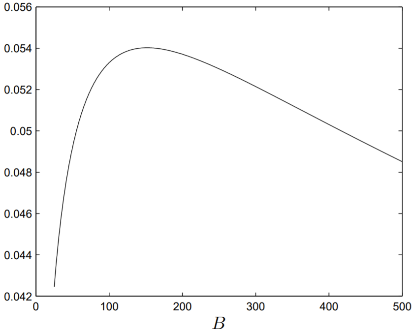
With the parameters \(d, g, p\), and \(m\) fixed, the integrated Euler-Lotka equation (2.7.6) is an implicit equation for \(r=r(B)\).

To demonstrate that \(r=r(B)\) has a maximum at some value of \(B\), we numerically solve (2.7.6) for \(r\) with the parameter values of \(g, p\) and \(m\) obtained from Table \(2.3\). Since \(r+d\) is maximum at the same value of \(B\) that \(r\) is maximum, and \(d\) only enters (2.7.6) in the form \(r+d\), without loss of generality we can take \(d=0 .\) To solve (2.7.6), it is best to make use of Newton’s method. We let

\[F(r)=(r+d) \exp [(g+B / p)(r+d)]-m\{1-\exp [-(B / m)(r+d)]\} \nonumber \]

and differentiate with respect to \(r\) to obtain

\[F^{\prime}(r)=[1+(g+B / p)(r+d)] \exp [(g+B / p)(r+d)]-\frac{B}{m} \exp [-(B / m)(r+d)] . \nonumber \]

For a given \(B\), we then solve \(F(r)=0\) by iterating

\[r_{n+1}=r_{n}-\frac{F\left(r_{n}\right)}{F^{\prime}\left(r_{n}\right)} \nonumber \]

Using appropriate starting values for \(r\), the function \(r=r(B)\) can be computed and is presented in Fig. 2.6. Evidently, \(r\) is maximum near the value \(B=152\), which is \(53 \%\) of the experimental value for \(B\) shown in Table \(2.3 .\)

Figure 2.6: A plot of \(r=r(B)\), which demonstrates that the Malthusian growth rate \(r\) is maximum near a brood size of \(B=152\)

Equation (2.7.13) contains the four parameters \(p, m, g\) and \(B\), which can be further reduced to three parameters by dimensional analysis. The brood size \(B\) is already dimensionless. The rate \(m\) at which eggs are produced and laid may be multiplied by the sperm production period \(s=B / p\) to form the dimensionless parameter \(x=m B / p\). The parameter \(x\) represents the number of eggs forgone because of the adult sperm production period and is a measure of the cost of producing sperm. Similarly, \(m\) may be multiplied by the larval growth period \(g\) to form the dimensionless parameter \(y=m g\). The parameter \(y\) represents the number of eggs forgone because of the juvenile growth period and is a measure of the cost of development. With \(B, x\) and \(y\) as our three dimensionless parameters, \((2.7.13)\) becomes

\[\frac{1}{B}\left(1+\frac{B}{x}\right)^{\frac{x+y}{B}} \ln \left(1+\frac{B}{x}\right)=\frac{B}{B+x} . \nonumber \]

Given values for two of the three dimensionless parameters \(x, y\) and \(B,(2.7.14)\) may be solved for the remaining parameter, either explicitly for the case of \(y=y(x, B)\), or by Newton’s method.

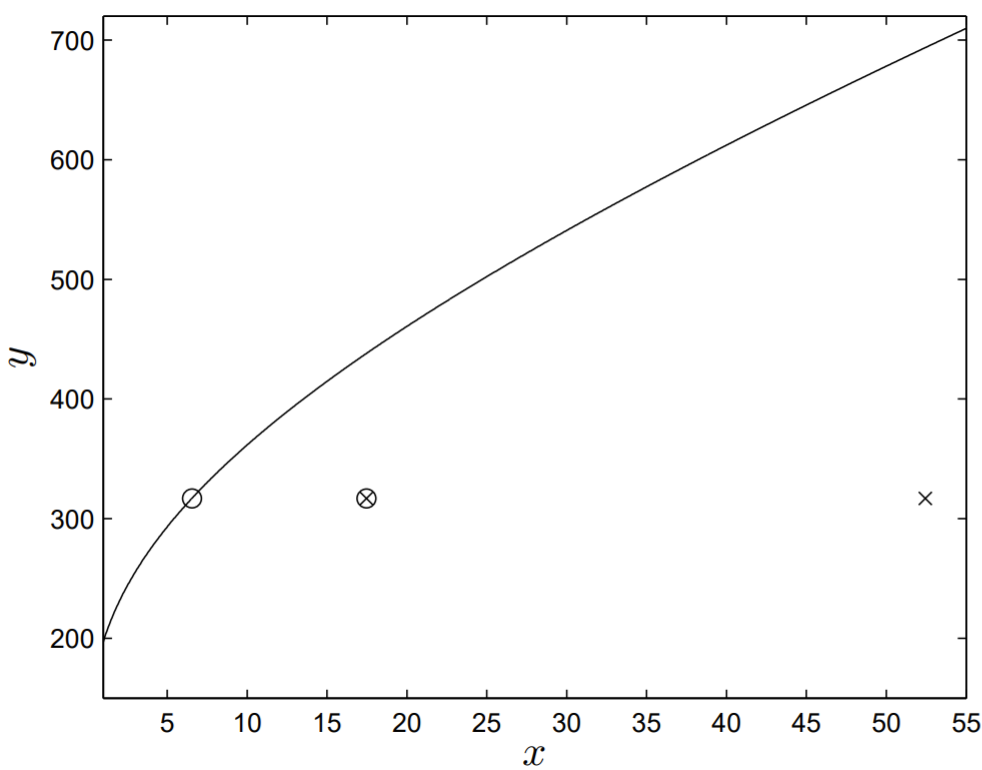
The values of \(x\) and \(y\) obtained from Table \(2.3\) are \(x=52.5\) and \(y=317\). With \(B=286\), the solution \(y=y(x)\) is shown in Fig. \(2.7\), with the experimental value of \((x, y)\) plotted as a cross.

The seemingly large disagreement between the theoretical result and the experimental data leads us to question the underlying assumptions of the model. Indeed, Cutter (2004) first suggested that the sperm produced precociously as a juvenile does not delay egg production and should be considered cost free. One possibility is to fix the absolute number of sperm produced precociously and to optimize the number of sperm produced as an adult. Another possibility is to fix the fraction of sperm produced precociously and to optimize the total number of sperm produced. This latter assumption was made by Cutter (2004) and seems to best improve the model agreement with the experimental data.

We therefore split the total sperm production period \(s\) into juvenile and adult

Figure 2.7: Solution curve of \(y\) versus \(x\) with brood size \(B=286\), obtained by solving (2.7.14). Values for \(B, m, p\) and \(g\) are taken from Table 2.3. The cross, crossed open circle and open circle correspond to \(y=m g\) and \(x=m f B / p\) with \(f=1,1 / 3\) and \(1 / 8\), respectively.

Figure 2.8: A more refined timeline of a hermaphrodite’s life.

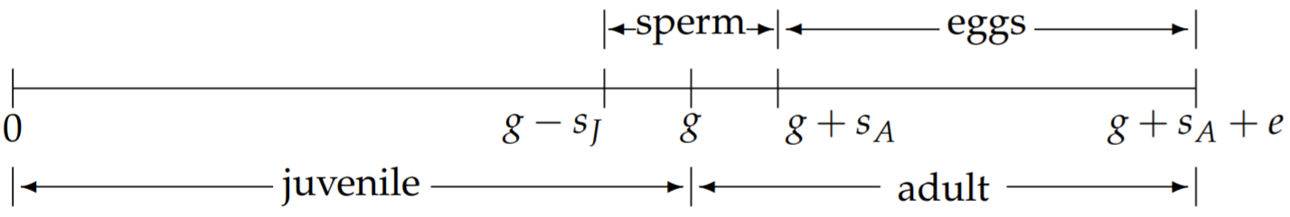
sperm production periods \(s_{J}\) and \(s_{A}\), with \(s=s_{j}+s_{A} .\) The revised timeline of the hermaphrodite’s life is now shown in Fig. 2.8. With the fraction of sperm produced as an adult denoted by \(f\), and the fraction produced as a juvenile by \(1-f\), we have

\[s_{J}=(1-f) s, \quad s_{A}=f s . \nonumber \]

Equation (2.7.4) for the age-specific maternity function becomes

\[m(a)= \begin{cases}m & \text { for } g+s_{A}<a<g+s_{A}+e \\[4pt] 0 & \text { otherwise }\end{cases} \nonumber \]

with

\[s_{A}=f B / p . \nonumber \]

The Euler-Lotka equation \((2.7.5)\) is then changed by the substitution \(p \rightarrow p / f .\) Following this substitution to the final result given by \((2.7.14)\) shows that this equation still holds (which is in fact equivalent to (12) of Chasnov (2011)), but with the now changed definition

\[x=m f B / p \nonumber \]

A close examination of the results shown in Fig. \(2.7\) demonstrates that near-perfect agreement can be made between the results of the theoretical model and the experimental data if \(f=1 / 8\) (shown as the open circle in Fig. 2.7). Cutter (2004) suggested the value of \(f=1 / 3\), and this result is shown as a crossed open circle in Fig. 2.7, still in much better agreement with the experimental data than the open circle corresponding to \(f=1\). The added modeling of precocious sperm production through the parameter \(f\) thus seems to improve the verisimilitude of the model to the underlying biology.