
4: Quantities in the Real World
- Page ID
- 57707

\( \newcommand{\vecs}[1]{\overset { \scriptstyle \rightharpoonup} {\mathbf{#1}} } \)
\( \newcommand{\vecd}[1]{\overset{-\!-\!\rightharpoonup}{\vphantom{a}\smash {#1}}} \)
\( \newcommand{\dsum}{\displaystyle\sum\limits} \)
\( \newcommand{\dint}{\displaystyle\int\limits} \)
\( \newcommand{\dlim}{\displaystyle\lim\limits} \)
\( \newcommand{\id}{\mathrm{id}}\) \( \newcommand{\Span}{\mathrm{span}}\)
( \newcommand{\kernel}{\mathrm{null}\,}\) \( \newcommand{\range}{\mathrm{range}\,}\)
\( \newcommand{\RealPart}{\mathrm{Re}}\) \( \newcommand{\ImaginaryPart}{\mathrm{Im}}\)
\( \newcommand{\Argument}{\mathrm{Arg}}\) \( \newcommand{\norm}[1]{\| #1 \|}\)
\( \newcommand{\inner}[2]{\langle #1, #2 \rangle}\)
\( \newcommand{\Span}{\mathrm{span}}\)
\( \newcommand{\id}{\mathrm{id}}\)
\( \newcommand{\Span}{\mathrm{span}}\)
\( \newcommand{\kernel}{\mathrm{null}\,}\)
\( \newcommand{\range}{\mathrm{range}\,}\)
\( \newcommand{\RealPart}{\mathrm{Re}}\)
\( \newcommand{\ImaginaryPart}{\mathrm{Im}}\)
\( \newcommand{\Argument}{\mathrm{Arg}}\)
\( \newcommand{\norm}[1]{\| #1 \|}\)
\( \newcommand{\inner}[2]{\langle #1, #2 \rangle}\)
\( \newcommand{\Span}{\mathrm{span}}\) \( \newcommand{\AA}{\unicode[.8,0]{x212B}}\)
\( \newcommand{\vectorA}[1]{\vec{#1}} % arrow\)
\( \newcommand{\vectorAt}[1]{\vec{\text{#1}}} % arrow\)
\( \newcommand{\vectorB}[1]{\overset { \scriptstyle \rightharpoonup} {\mathbf{#1}} } \)
\( \newcommand{\vectorC}[1]{\textbf{#1}} \)
\( \newcommand{\vectorD}[1]{\overrightarrow{#1}} \)
\( \newcommand{\vectorDt}[1]{\overrightarrow{\text{#1}}} \)
\( \newcommand{\vectE}[1]{\overset{-\!-\!\rightharpoonup}{\vphantom{a}\smash{\mathbf {#1}}}} \)
\( \newcommand{\vecs}[1]{\overset { \scriptstyle \rightharpoonup} {\mathbf{#1}} } \)
\(\newcommand{\longvect}{\overrightarrow}\)
\( \newcommand{\vecd}[1]{\overset{-\!-\!\rightharpoonup}{\vphantom{a}\smash {#1}}} \)
\(\newcommand{\avec}{\mathbf a}\) \(\newcommand{\bvec}{\mathbf b}\) \(\newcommand{\cvec}{\mathbf c}\) \(\newcommand{\dvec}{\mathbf d}\) \(\newcommand{\dtil}{\widetilde{\mathbf d}}\) \(\newcommand{\evec}{\mathbf e}\) \(\newcommand{\fvec}{\mathbf f}\) \(\newcommand{\nvec}{\mathbf n}\) \(\newcommand{\pvec}{\mathbf p}\) \(\newcommand{\qvec}{\mathbf q}\) \(\newcommand{\svec}{\mathbf s}\) \(\newcommand{\tvec}{\mathbf t}\) \(\newcommand{\uvec}{\mathbf u}\) \(\newcommand{\vvec}{\mathbf v}\) \(\newcommand{\wvec}{\mathbf w}\) \(\newcommand{\xvec}{\mathbf x}\) \(\newcommand{\yvec}{\mathbf y}\) \(\newcommand{\zvec}{\mathbf z}\) \(\newcommand{\rvec}{\mathbf r}\) \(\newcommand{\mvec}{\mathbf m}\) \(\newcommand{\zerovec}{\mathbf 0}\) \(\newcommand{\onevec}{\mathbf 1}\) \(\newcommand{\real}{\mathbb R}\) \(\newcommand{\twovec}[2]{\left[\begin{array}{r}#1 \\ #2 \end{array}\right]}\) \(\newcommand{\ctwovec}[2]{\left[\begin{array}{c}#1 \\ #2 \end{array}\right]}\) \(\newcommand{\threevec}[3]{\left[\begin{array}{r}#1 \\ #2 \\ #3 \end{array}\right]}\) \(\newcommand{\cthreevec}[3]{\left[\begin{array}{c}#1 \\ #2 \\ #3 \end{array}\right]}\) \(\newcommand{\fourvec}[4]{\left[\begin{array}{r}#1 \\ #2 \\ #3 \\ #4 \end{array}\right]}\) \(\newcommand{\cfourvec}[4]{\left[\begin{array}{c}#1 \\ #2 \\ #3 \\ #4 \end{array}\right]}\) \(\newcommand{\fivevec}[5]{\left[\begin{array}{r}#1 \\ #2 \\ #3 \\ #4 \\ #5 \\ \end{array}\right]}\) \(\newcommand{\cfivevec}[5]{\left[\begin{array}{c}#1 \\ #2 \\ #3 \\ #4 \\ #5 \\ \end{array}\right]}\) \(\newcommand{\mattwo}[4]{\left[\begin{array}{rr}#1 \amp #2 \\ #3 \amp #4 \\ \end{array}\right]}\) \(\newcommand{\laspan}[1]{\text{Span}\{#1\}}\) \(\newcommand{\bcal}{\cal B}\) \(\newcommand{\ccal}{\cal C}\) \(\newcommand{\scal}{\cal S}\) \(\newcommand{\wcal}{\cal W}\) \(\newcommand{\ecal}{\cal E}\) \(\newcommand{\coords}[2]{\left\{#1\right\}_{#2}}\) \(\newcommand{\gray}[1]{\color{gray}{#1}}\) \(\newcommand{\lgray}[1]{\color{lightgray}{#1}}\) \(\newcommand{\rank}{\operatorname{rank}}\) \(\newcommand{\row}{\text{Row}}\) \(\newcommand{\col}{\text{Col}}\) \(\renewcommand{\row}{\text{Row}}\) \(\newcommand{\nul}{\text{Nul}}\) \(\newcommand{\var}{\text{Var}}\) \(\newcommand{\corr}{\text{corr}}\) \(\newcommand{\len}[1]{\left|#1\right|}\) \(\newcommand{\bbar}{\overline{\bvec}}\) \(\newcommand{\bhat}{\widehat{\bvec}}\) \(\newcommand{\bperp}{\bvec^\perp}\) \(\newcommand{\xhat}{\widehat{\xvec}}\) \(\newcommand{\vhat}{\widehat{\vvec}}\) \(\newcommand{\uhat}{\widehat{\uvec}}\) \(\newcommand{\what}{\widehat{\wvec}}\) \(\newcommand{\Sighat}{\widehat{\Sigma}}\) \(\newcommand{\lt}{<}\) \(\newcommand{\gt}{>}\) \(\newcommand{\amp}{&}\) \(\definecolor{fillinmathshade}{gray}{0.9}\)In this course, we seek to solve practical problems in natural resource management and ecology, but we focus on the use of quantitative tools in service of this objective. Before diving too deeply into problem-solving, we should ensure that we know what is meant by quantities, quantitative tools, and quantitative reasoning. We will also establish a few conventions for how quantities are represented in science and how quantitative information can be most effectively communicated.
4.1 Quantities in Natural Resources
If we can assess the presence or absence of something, count its number, measure some property that it has, or compare it to another object, it can be quantified. That quantified thing is then represented by a quantity that is itself now a property of the quantified thing. If that sounds confusing, read on to some of the examples below. A fully-defined quantity has five components:
- Name: what we call it.
- Procedural statement: how it is measured or computed.
- Number: numerical value(s) corresponding to magnitude or multitude.
- Units: how it is scaled.
- Symbol: a character that stands for the quantity in equations.
Defining a quantity might seem somewhat pedantic, but it has important implications for what we can and cannot do with it. This contrasts fundamentally with the abstract variables we encountered in high school math. In that setting, there is rarely any reason to question whether it is OK and meaningful to add 3x and 8y, we just do what we’re asked. But in the world of real quantities, if x stands for “milligrams of sodium chloride” and y stands for the number of eggs in a Northern Cardinal’s nest, it’s not so clear that we can perform that addition. Even if we do, it is not so clear what the result means.
In the introductory chapter, we pondered the Iowa DNR’s roadside pheasant survey and what it means for pheasant populations across the state. The pheasant count yields a single number each year, for example 23.9 individuals per 30 miles in 2015. We discovered what this quantity means and how it is measured in the Introduction, so we already have most of the ingredients of a fully-defined quantity. We only need a symbol. This is a pretty trivial step in simple problems, where the primary constraint is to make the symbol unambiguous and suggestive of the quantity it represents. Perhaps we should then choose P for our symbol. If we were to prepare a document describing the DNR roadside pheasant survey, once we establish each of the five properties\(^{1}\) of our quantity, we can thereafter use P with confidence that the information conveyed by that symbol is clearly established: within the context of our document, P would refer to the series of annual estimates of pheasant density according to the method established by the DNR. This formality thereby provides a shorthand name and eliminates any ambiguity in discussion of quantities. Note that this is different than P, which we used previously as the chemical symbol for the element Phosphorus. If we happened to be working on a problem involving both pheasants and Phosphorus, we might select our symbol differently to avoid ambiguity.
\(^{1}\)Name, procedural statement, number, units, and symbol
As we indicated above, there are many types of quantities that we encounter in science. We can treat presence/absence information as a quantity, measured with a nominal scale\(^{2}\). Was there a black-capped chickadee on the bird feeder at 3:30 PM? Is there a beetle in the pit-trap we set up in a field? An ordinal scaled quantitiy is one in which individual measurements or components are ranked or ordered.
In what order did different birds arrive at and depart from the bird feeder\(^{3}\)?
\(^{2}\)Nominal-scaled quantities take the form of categories; a few pairs of categories that fit this definition might be present or absent; infected or not infected
\(^{3}\)Ordinal-scaled quantities have values according to their rank among the population or data.
In the above cases, distinctions between the scales are clear and obvious, but in others they can be more subtle. Consider the expression of the quantity temperature. We have several scales we can choose from for measuring and expressing temperature. Most important and familiar are the Fahrenheit, Celsius (Centigrade), and Kelvin (absolute) scales. The Celsius scale, for example, is defined according to the freezing and boiling points of water, and the temperatures that those phenomena corresponded to were defined to have values of 0\(^{◦}\)C and 100\(^{◦}\)C, respectively. A degree of Celsius is therefore defined on an interval scale\(^{4}\), where a unit of temperature change is 1/100th of the difference between the boiling point and freezing point of water. In contrast, Kelvin is a measure of the absolute thermal energy contained in a substance, in reference to a theoretical state of zero energy\(^{5}\).
\(^{4}\)Interval-scaled quantities may take negative values.
\(^{5}\)the Kelvin scale, named for Lord Kelvin (William Thomson), is considered an absolute temperature scale, measuring the absolute thermal energy in a substance.
Kelvins are a ratio scale , with a natural zero point and a unit magnitude that represents the value on a scale relative to that zero point. It can be confusing to distinguish between interval and ratio scaled quantities, but the following example might help illuminate the difference. Imagine that you measured a lake’s surface water temperature at one moment in mid March to be 1\(^{◦}\)C. Now suppose you returned a week later to find that the temperature has increased to 2\(^{◦}\)C. Wow, the temperature doubled, since 2 is twice as large as 1! Well, no it didn’t. Because Celsius is an interval scale, chosen arbitrarily to have a value of zero at the freezing temperature of water, we cannot say it doubled. The issue with this might be even more clear if our first measurement had been -0.1\(^{◦}\)C (supercooled!) instead of 1\(^{◦}\)C. Then if we apply the same logic as before to characterizing the change to 2\(^{◦}\)C, we would have to say that the temperature is -20 times the initial value, which is ridiculous. It’s ridiculous because our scale does not have a natural zero point, and instead describes interval differences between a measured temperature and a standardized reference point. In contrast, a temperature of 300 K is actually twice as hot as a temperature of 150 K, since this is a ratio scale\(^{7}\).
\(^{6}\)Ratio-scaled quantities cannot have negative values; a non-positive value indicates an absence of the quantity.
\(^{7}\)For additional topical perspective on quantities and scaling in ecology, consult a resource like Schneider, D.C., 2009, Quantitative Ecology, 2nd ed., London, UK, Academic Press, 415 p.
It might seem a bit esoteric to define quantities and their unit scales in so much detail, but hopefully you can now see how different scales might entail different rules for what manipulations are or are not meaningful.
4.2 What Quantitative Reasoning Is
Using, manipulating, and interpreting quantitative information are the prerogative of professional scientists and natural resource managers. The term quantitative reasoning is often used to describe the processes of constructing and making sense of contextualized quantitative information\(^{8}\). When we look for patterns in water quality data, interpret pheasant population trends, or estimate the number of person-hours required for removal of invasive shrubs in a forest, we are applying quantitative reasoning. An individual’s aptitude for quantitative reasoning is sometimes referred to as quantitative literacy.
\(^{8}\)One researcher describes quantitative reasoning as “sophisticated reasoning with elementary mathematics, rather than elementary reasoning with sophisticated mathematics.” (Steen, L., 2004, Achieving Quantitative Literacy: An Urgent Challenge for Higher Education, Washington, DC, MAA.)
A guiding premise of this book is that the lifetime value of strong quantitative literacy is greater than that of pure mathematics for natural resource professionals. To be sure, basic mathematical skills are fundamentally essential for quantitative reasoning. But for most professionals outside of engineering and the physical sciences, these skills are mostly learned in secondary school math. What often isn’t learned is how to use those skills to make sense of things in the world around us.
4.3 Units & Dimensions
Quantities with practical meaning to us will often have units. Consider a few random examples:
- 71 foot tall tree
- 16.4 grams of soil
- 42 snow geese
- 39 breaths per minute
- 385 ppm carbon dioxide
Each of these examples would lose much of their meaning if we only stated the number and not what the number corresponded to: 71, 16.4, 42, 39, 385. We can certainly plug these numbers into equations and work with them in a purely mathematical sense, but they probably no longer have a meaning that we care about. Thus, we need to keep track of units. Units can be any standard template or scale according to which we measure a quantity. A foot, for example, though originally loosely defined by the length of a Greek or Roman man’s foot, is now defined with reference to a meter, which in turn is defined according to the distance light travels in a vacuum during a pre-defined time period. Likewise, grams and minutes are units of mass and time defined according to internationally standardized references.
Paying attention to units and dimensions is not mere formality. In the scaled quantities we use in science, units and dimensions constrain what mathematical operations are permissible.
Dimensions are sometimes conflated with units, but the term is distinct and more broad. In casual usage, the term “dimensions” of- ten implies that we wish to know how large something is - in other words, its length, area or volume. In the physical sciences, dimensions are a way to group different types of units that can be simply scaled with one another. Inches and centimeters are both lengths. No matter what object you measure – perhaps a young brook trout’s total length – if it is an inch long, it is by simple unit conversion also 2.54 centimeters long. Both are units of length. But just because I find that the fish is 1 inch or 2.54 centimeters long, that does not necessarily tell me how heavy it is. So mass is a different fundamental dimension than length, and whether I measure mass in grams or slugs, it has dimensions of mass. In fact, most of the quantities that scientists deal with are composites of only three fundamental dimensions: mass, length, and time. Sometimes we use the symbols [M], [L], and [T] in square brackets to denote when we are talking about dimensions. We can also have dimensionless quantities which we can (for reasons that we’ll see below) denote with [1], and which we’ll often encounter when we are dealing with nominal, ordinal, or multitude scales.
Most quantities in the natural sciences have dimensions involving mass [M], length [L] and time [T]
A quantity made up of any combination of the fundamental dimensions can be called a derived quantity. Speed is an example of a derived quantity because it implicitly contains two quantities, a distance or length traveled during a period of time, [L T\(^{−1}\)]. Note that we haven’t said whether we are measuring length in meters or feet or whatever, nor have we said that time is in seconds or hours or millennia. Dimensions are more like categories of units, and we can convert from one set of units to another within each category by performing multiplication or division. Energy is also a derived quantity, and can be expressed in units of Joules or Calories. But regardless of the units employed, any quantity of energy has dimensions of [ML\(^{2}\)T\(^{−2}\)]. We just need to be careful if we are working with equations that we don’t mix units, or we’ll be left with gobbledygook.
4.4 Comparing apples and oranges
We all learn in junior high or high school science to pay attention to units, and for good reason. Keeping track of units and making sure that our units are consistent in any computation we do with physical quantities can prevent costly mistakes. I’m not terribly pleased about it, but I probably spend a few hours a month painstakingly performing unit conversions in my research – indeed it may be the most frequent type of computation I do, but I do it because I know it is important.
Let’s consider a simple contrived example, similar to one that we will encounter later this semester: suppose you are told that the soil in your back yard has 15.84 ounces of lead per metric ton of soil. Should you worry? Well, according to EPA guidelines, remediation is recommended if lead concentrations in residential yards exceed 400 parts per million. Parts per million is a dimensionless unit similar to a percent but much smaller and it can correspond to a mass (or volume) of one substance contained in a mass (or volume) of some mixture of substances. Our measurements are already both masses, so 15.84 ounces/1 ton is [MM\(^{−1}\)], and is already dimensionless, but our units are not consistent. We could fix this in several different ways, but one simple one might be to convert tons of soil to ounces, so that we have ounces over ounces, yielding consistent units. We could spend lots of time (not wisely, I would argue) setting up fractions on paper to figure this out (how many ounces in a pound, how many pounds in a kilogram, how many kilograms in a ton. . . ), but as long as we have access to a computer we might as well use it. Plenty of apps and websites will do basic unit conversions for you, including google itself. Employing one of these, we see that there are 35274 ounces in a metric ton, and now we can express our measured concentration as 15.84 ounces / 35274 ounces, or about 0.00045. To convert from this decimal value to parts per million, we just need to multiply by one million or 106 (much like you would multiply by 100 to get a percent), giving us roughly 450 ppm lead. So at 450 ppm, the lead concentration in our soil exceeds the threshold that the EPA has deemed safe, but is not cause for great alarm.
4.5 Problem solving without numbers
Dimensions are so useful in science and engineering that there are entire subdisciplines devoted to dimensional analysis. While these folks are usually using dimensional analysis as a technique for extracting relationships between variables in complex equations that cannot be solved directly, we can also use dimensions to help solve simpler problems and catch errors or inconsistencies. This is because physically-meaningful equations that describe relationships between quantites must be dimensionally homogeneous\(^{9}\).
\(^{9}\)Dimensional homogeneity requires equations, if expressed only in terms of the units representing each quantity, to remain equal
That is, the dimensions on one side of the equation must be the same as those on the other side. If we know the units of every quantity in a mathematical relationship and can figure out the corresponding dimensions, we can compare dimensions on either side of the equation to verify that it is dimensionally homogeneous. This can feel a lot like solving an algebraic equation without actually using any numbers, just combinations of [M], [L] and [T]. Doing this after making some algebraic manipulations on an equation is a handy way of checking for mistakes! Similarly, if we are uncertain of the dimensions of a constant or variable in an equation, we can solve for that constant on one side of the equation and the dimensional grouping on the other side, through the requirement of dimensional homogeneity, will apply to the unknown.
In constructing or manipulating algebraic relationships, enforcing and verifying dimensional homogeneity can yield insights and catch errors.
Rules for algebraic manipulation of dimensions are straightforward. Multiplying, dividing, or raising to a power any quantities of any dimensions is permissible, and the resulting quantity has dimensions that are the appropriate product, quotient, or power of the original dimensions. Adding and subtracting may only be done between quantities with identical dimensions (and later you should verify that the units are also identical). Let’s consider an example where we wish to find the dimensions of the entities in a simple equation describing the accumulation over time of insects (measured in mass) in a pit trap:
m = m\(_{0}\) + kt (4.1)
where we know m is mass and so has dimensions [M] and t is time and so has dimensions [T]. What are the dimensions of the other two variables? Well, assuming the equation is dimensionally homogeneous and knowing that the left-hand side has dimensions [M], the right-hand side must work out to have dimensions of [M] as well. Furthermore, since added quantities must have identical dimensions, we know that each of the two terms added together on the right hand side must have dimensions of [M]. So m\(_{0}\) is a mass, and k must be something that, when multiplied by a time with dimensions [T], gives a mass. Therefore, k must have dimensions of [MT\(^{−1}\)], or mass per time.
Rearranging equations algebraically with only dimensions or units rather than numbers is a useful way to find the units or dimensions of unknown variables.
4.6 Communicating Quantitative Information
We all construct our understanding of quantitative information a little bit differently. I personally grasp quantitative patterns or rela- tionships best if I see it in a graph. Others might have an easier time reading or listening to a verbal description of patterns and relation- ships. Still others will be more moved by equations or lists of num- bers. We can understand and communicate quantitative information in all of these ways – and maybe more (we can encode quantitative information in sound, right?)! But to be well-rounded scientists and managers, we must be able to create and interpret each form. The diagram in Figure 4.1 illustrates these four ways of communicating quantitative information.
Here’s what each of the nodes of the triangle mean:
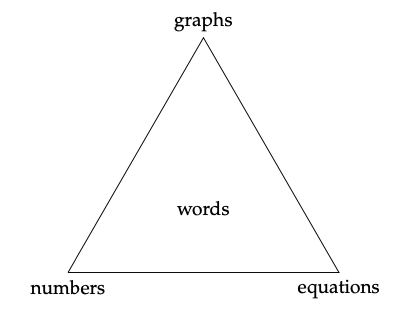
Figure 4.1: Ways of communicating and understanding quantitative information.
• Graphs, images, figures: any visual display of quantities or relationships between them. Single-variable statistical charts (e.g., histograms) and two-dimensional graphs (i.e., x-y scatter-plots) will be the most frequently encountered, but maps are another example. Often the most efficient way to demonstrate patterns or large volumes of data.
- Numbers, in lists or tables: for numerical information, the most direct, precise, and unambiguous way of communicating quantities that aren’t too numerous (i.e., a short list).
- Equations, inequalities, or proportionalities: a formal and precise way to state hypothesized, derived, or observed relationships between quantities.
- Words, concepts: descriptions and interpretations, either standing alone or to accompany another form of expression.
In technical reports, it is good practice to employ at least two or three forms of quantitative expression, where one form will always be words. Words are in the center of the triangle because they must be used to link the other forms conceptually, and without them we cannot claim to be understanding and communicating effectively. Furthermore, as professionals, we cannot simply provide charts or tables of data and expect them to speak for themselves. Part of the role of scientists and managers is to interpret quantitative information and make decisions or recommendations based on our interpretations.
4.6.1 Example: brook trout recruitment (teaser Problem 3.7)
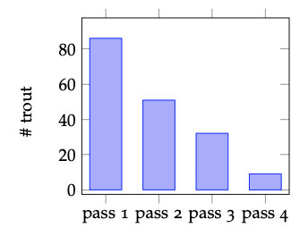
Figure 4.2: Bar chart showing the number of brook trout removed from a stream reach during each of four consecutive electrofishing passes.
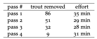
Table 4.1: Brook trout removal from four electrofishing passes in one stream reach, including information about
the number of minutes (effort) elapsed during each pass.
The data from electrofishing studies of fish population and age-structure can be quite simple. A typical set-up would begin with blocking the channel upstream and downstream with fences or nets to prevent fish from entering or leaving the study reach. Then fisheries technicians would slowly traverse the study reach with one person applying the electrodes through the water and a second collecting the stunned fish into a bucket or live well. Captured fish are then measured, weighed, aged (if desired) and returned to the water. In depletion surveys, the fish are returned upstream or downstream of the blocking nets, so as to avoid immediate re-capture. Subsequent passes would operate similarly, and the presumption is that with each removal, the number of fish remaining in the study reach is diminished. Figure 4.2 and Table 4.1 both show data from four consecutive passes through a small trout stream. The bar graph (Figure 4.2) provides a very simple visual indication of the change in the number of fish captured in each pass. Graphs like this can be extremely valuable for efficiently conveying trends or relationships between quantities. However, they often don’t allow readers or viewers to know precisely what the values of the shown quantities are. Furthermore, graphs with too many different variables can become overly complex. If we wish to communicate precise values of quantities, particularly where there are multiple different kinds of variables, data tables like Table 4.1 are perhaps the best option.
Given only the information presented already about the brook trout electrofishing catch, communicating through equations is probably unwarranted. However, a textual narrative is essential for communicating the nature and meaning of the data presented in this example. Suppose you were unfamiliar with electrofishing and depletion methods for fish population assessment, would the bars in Figure 4.2 and the numbers in Table 4.1 tell a clear story? The figure captions and the paragraphs above are essential for drawing meaning from the figure and table. This is why words are at the center of the triangle in Figure 4.1. And this is also why it quantitative problem solving is a writing-intensive endeavor. If we are unable to communicate clearly about our ideas, strategies, results, and conclusions, most of the effort is for naught.
1. From our bulleted list of examples at the beginning of section 4.3, what are the units and dimensions for each quantity? Write them with square-bracket notation.
2. In population studies, it is recognized that the number of individ- uals captured depends strongly upon how much time (effort) is spent in active pursuit. As a result, a better variable to quote than the number of trout caught is the number of trout per unit effort, or catch-per-unit-effort (CPUE). If one minute is defined as the ba- sic unit of effort for the data in Table 4.1, convert the data to a new variable, catch (trout removed) per unit effort (minute). Plot the result in a bar graph similar to Figure 4.2 and create a table with this additional variable alongside the other three.
3. What are the dimensions of the new variable created in #2?
4. What kind of quantity is shown on the horizontal axis of Fig- ure 4.2? How do you think this constrains appropriate ways to visualize these data graphically?