5: Working with Numbers

Among the most fundamental operations we do with quantities is arithmetic. We can encounter the need for arithmetic in any phase of problem solving, from making a ballpark estimate in the Under- stand phase to computing and double-checking a final result in the Execute and Check phases. Once we have a solid grasp of the operations that are allowable and those that aren’t – for example, is it OK to add or subtract quantities expressed in different units or on different scales? – we may get down to business with performing basic operations.

Arithmetic

Arithmetic according to Wikipedia: a branch of mathematics that consists
of the study of numbers, especially the properties of the traditional operations on them – addition, subtraction, multiplication and division.

Most of us probably feel comfortable with most of these operations, at least when they concern simple numbers. However, it becomes easy to make errors or overlook important steps when we’re dealing with extremely large or small numbers, or when unit con- versions become necessary. One setting in which we often encounter such difficulties is in working with proportions, including concentrations, ratios, and percentages. Though quantities like these are often conceptually simple, working with them and converting among ways of expressing them can be challenging. This chapter highlights some concepts and techniques for working with these sorts of unwieldy numbers so that we can work confidently, avoid simple mistakes, and even catch more complex ones.

We begin with a method for doing arithmetic that can be used to simplify computations, or to approximate solutions when a back-of- the-envelope computation is all you need. The method is particularly powerful when computations involve very large or very small num- bers. As such, it can be useful for making ballpark estimates in the early stages of problem-solving. Our method makes strategic use of scientific notation, which you’ve probably encountered in sec- ondary science classes. The philosophical basis of scientific notation also leads to the notion of order of magnitude, a concept that can be useful for comparing quantities as well as for judging the the ap- propriateness of estimates. Along the way, we’ll compare some ways of expressing normalized quantities like concentrations and propor- tions, and review the rules for arithmetic with exponents.

5.1 Scientific Notation

In high school chemistry, we learn that there are more than 602 sex-tillion molecules in a mole of a chemical substance\(^{1}\). But we don’t normally see Avogadro’s constant written as some number of sextillions, nor do we see it elaborated with all of the 24 digits necessary to write it in integer form: it is difficult to keep track of all those digits when writing them, and even more difficult to keep track when you’re reading or comparing different numbers. Instead of writing the entire number out, we use the shorthand of scientific notation, where Avogadro’s constant looks more like 6.022×10 . In general, scientific notation has the form:

a = 10\(^{b}\)

Element 1.

\(^{1}\)602 sextillion, or 6.022×10\(^{23}\) is Avogadro’s constant, the number of molecules in one mole of a chemical substance

where a and b are sometimes called the mantissa and power, respectively. So Avogadro’s constant has a mantissa of about 6.022 and a power of 23, which is equivalent to saying that the complete quantity has 23 digits after the mantissa\(^{2}\). Obviously this is a very large number. We can just as easily express very small numbers with scientific notation. An e. coli bacterium is roughly 2 μm (micrometers) long, which is 2×10−6m. Here, the power of −6 indicates not that it’s a negative number (it would be absurd to say something has a negative length, because length is a ratio scale!), but that it is smaller than 1 and that there should be 6 digits to the right of a decimal point if we wished to express it as a decimal number. So we could express this equivalently in a few ways:

2μm = 0.000002m = 2 × 10\(^{−6}\)m.

Element 2.

\(^{2}\)A related issue is that of significant digits. Scientific notation allows us to clearly specify how precise we are claiming to be through the number of digits included in the mantissa: in this case, 4.

Note that these equalities both amount to unit conversions, but the second equality is specifically a conversion to scientific notation. Negative exponents indicate numbers smaller than 1, and there are occasions where it can be helpful at times to can write these as fractions. When we have a quantity expressed in scientific notation with a negative exponent 10\(^{−b}\), that is equivalent to the same quantity divided by 10\(^{b}\). Therefore, another way to express the length of e.coli is:

\(2 \times 10^{-6} \mathrm{~m}=2 \times \frac{1}{10^{6}} \mathrm{~m}\)

Element

In the standard order of operations, parentheses take precedence, then exponents, then multiplication or division, and finally addition and subtraction.

So dividing by 10\(^{6}\) is the same as multiplying by 10\(^{-6}\). Notice here that the order of operations is important. By convention, exponents take precedence over multiplication, division, addition and subtraction. So we don’t divide by the mantissa (2) when we express this quantity in fractional terms because the only thing that is raised to the exponent is the base, in this case 10. We could, however, move the mantissa to the denominator with its 10\(^{6}\) by taking its reciprocal, right? That’s another way of invoking the old grade-school rule: dividing by a number is the same as multiplying by it’s reciprocal. In this case, we’d end up with an equivalent value for the length of e. coli that looks like

\(2 \times 10^{-6} \mathrm{~m}=\frac{1}{0.5 \times 10^{6}} \mathrm{~m}=\frac{1}{5.0 \times 10^{5}} \mathrm{~m}\)

Notice that in the last step we’ve borrowed a “ten” from the power to make the mantissa greater than 1: this is by convention . A general rule for expressing a quantity in scientific notation is to have one nonzero digit before the decimal point in the mantissa, and as many significant figures as appropriate for the problem to the right of the decimal. So we could express the e. coli length as 0.2×10\(^{−5}\)m or 200×10\(^{−8}\)m, but in most cases that is bad form. We shall see below, however, there are times when doing arithmetic by hand can be simplified by temporarily expressing quantities in such an unconventional way.

Element 3.

\(^{3}\)Quantities expressed in scientific notation should have one nonzero digit to the left of the decimal point.

A useful concept in working with really large or really small numbers is the order of magnitude of a quantity. In obtaining a ballpark estimate of a quantity or in computing something using only very rough approximations for the input values, it may be unnecessary or inappropriate to worry about being off by a factor of 2 or so. We might be satisfied knowing that the result is “a few thousand” or “a coupe hundredths”. If we’re using scientific notation, this is equivalent to ignoring the mantissa and just citing the base and power. So instead of saying that an e. coli is 2×10\(^{−6}\)m, we can say it is on the order of 10\(^{−6}\)m long. This kind of reasoning is particularly useful in comparing multiple quantities. A grain of coarse sand, for example, is on the order of 10\(^{−3}\)m in diameter, so it is three orders of magnitude larger (−3 is three more than −6) than an e. coli bacterium. Once we wrap our minds around what that means (three orders of magnitude is a factor of 103, or a thousand!), comparisons can be enlightening in assigning quantitative “importance” to different variables in an equation.

Element

The order of magnitude of a quantity is essentially the value of the exponent when expressed in scientific notation.

The fact is, in normal communication about the length of e. coli, we’d probably stick with 2 μm as a clear way to express it in written text. Most of the alternative ways above are more clumsy in writing, and certainly the last few equivalent expressions above are not intuitive (we only went there to demonstrate the technique!). Quantities expressed in scientific notation should have one nonzero digit to the left of the decimal point. The order of magnitude of a quantity is essentially the value of the exponent when expressed in scientific notation. However, in comparisons with other qantities or when performing computations with other quantities that are expressed in different units, it is usually smart to convert all quantities to a uniform system of units, like the systeme internationale, or SI.

5.2 Normalized quantities

In the sciences, normalization of quantities often refers to the process of dividing some scaled quantity by a standard, total, or reference value of the same quantity. Consider some schemes form normalization that you are already very familiar with. A percentage is a normalized quantity, determined by dividing some number that represents a subset of a larger collection by the total number in the collection and then multiplying by 100%. For example, suppose we have tested 360 white-tail deer carcasses (from road-kill and hunter harvest) for chronic wasting disease (CWD) and find that 83 are positive. Given this data, we can all agree that the percent of the sampled population infected with CWD is:

\(\frac{83}{360} \times 100 \%=23.0556 \%\) (5.1)

En route to computing this, we created the ratio 83 to 360, which is around 0.23 if you simplify it with your calculator. As with many such ratios, we can choose from a variety of different but equivalent ways of expressing this quantity. We could just express it as the ratio of two whole numbers like 83:360\(^{4}\), or as the fraction:

\(\frac{83}{360}\). (5.2)

Element 4.

\(^{4}\)this is the way we usually express a map scale, like 1:24,000. See Part III of this book for more on that issue.

Or as we’ve already seen, it is simple to write it as a decimal number (0.230556). But since we encounter percentages frequently, we may more readily appreciate it expressed as a percentage. For the present purposes, we could describe a percentage as “parts per hundred”, since it is just the same ratio scaled to an arbitrary reference value of 100. In other words, for every hundred deer in the sample, about 23 have CWD. Expressing a quantity in “per mil” is closely analogous, except instead of multiplying by the factor 100% we’d multiply by 1000(that’s the per mil symbol)\(^{5}\). In this case, we’d end up saying that about 83/360 ×1000 = 231(or 231 per thousand deer) are infected. To make this even more absurd, we could express the same information just as easily as parts per million (ppm) or parts per billion (ppb) following a similar tactic. Each of these ways of expressing a normalized quantity is arithmetically equivalent, but implies a different realm of precision about the quantity of interest and the scope of its possible values. We’d likely never talk about deer in parts per million, but we might talk about lead concentrations that way!

Element 5.

\(^{5}\)Although not common in many disciplines, isotope concentrations are often expressed in %, where the reference value is the isotopic ratio of a standard substance.

Other types of normalized quantities in science include frequencies, concentrations, and probabilities, to name a few. The quantities may be expressed somewhat differently, but in most cases there is a comparison being made between values of the same dimensions (and often the same units!). Indeed this is sometimes a simplifying strategy: when you normalize a quantity to a standard of the same units, details about the specific units by which the quantities were measured can be discarded. Often this is a good thing. For example, when we use a map that is scaled at, for example, 1:24,000, we are not told what units that ratio was constructed with, because it doesn’t matter! If you use a ruler to find that the map distance be- tween two features on the map is 2 inches, that distance in the real world is equal to 2 × 24, 000 = 48, 000 in. It doesn’t matter whether your ruler is ruled in inches, centimeters, furlongs or rods, the quantity you measure on the map only needs to be multiplied by the scale factor (24,000) to find the true distance! As we’ve seen, however, neglecting the specific units used to derive a normalized quantity can also be the cause of some confusion (is the concentration of one sub- stance mixed with another computed on the basis of their masses, volumes, or something else?). It becomes a good thing if the procedural statement for the quantity is either made clear or is known by convention.

How do we use a normalized quantity to our advantage? Suppose I extrapolate from our sample of CWD in deer carcasses to predict that 23% of the deer in the entire county are infected with CWD. If we take for granted that my science is good, all we need to know to find out the number of CWD-infected deer in the county is the total number of deer in the county, N\(_{deer}\). Once we recognize that the ratio of infected deer to total deer is 0.23 (23% of the total population of 100%), we need only perform a simple multiplication:

\(\frac{N_{CWD}}{N_{deer}}\) = \(\frac{23%}{100%}\) = 0.23 (5.3)

N\(_{CWD}\) = 0.23N\(_{deer}\) (5.4)

Thus, the benefit of expressing the number of infected deer as a normalized quantity (assuming our 23% assertion is accurate) is its generality. We can write a simple relationship like Equation 5.4 and, as long as the relationship remains valid, apply it on any relevant scale\(^{6}\). The process of re-scaling a ratio (or other normalized quantity) is sometimes called proportional reasoning, and is one of the key strategic processes in probability, and as we’ll see in the next chapter, it is the foundation of much of trigonometry. The construction of abstract triangles in the service of problem-solving is usually a means of comparing the ratios of two lengths or distances.

Element 6.

\(^{6}\)Recognizing how far one can safely scale up from a representative sample is a rich, but complex issue.

There are some oddball normalized quantities in science that are frequently expressed in inhomogeneous units, either as a consequence of their very high or low intrinsic magnitudes or due to the procedure used to measure them. One example is slope in the con- text of river channels or footpaths, which are often less than 1%. Because typical channel slopes are so small, it is common to see slopes expressed in units of “feet per mile” or “meters per kilometer”. They are still normalized quantities, but the inhomogeneous units must be stated explicitly. Similarly, concentrations of solutes or suspensions are sometimes expressed in units like mg/L (milligrams per liter), where the dimensions are a weight per volume. This is convenient because of the relative simplicity of weighing a solid component added to (or isolated from) a volume of liquid. On the other hand, concentrations of substances like dilute hydrochloric acid (HCl; often used in soil chemistry) are are often described as percentages: 5% HCl usually means a mixture in which 5% of the total volume is pure HCl and the remaining (100-5)% = 95% is pure water. Again, this makes sense because when mixed, both components are liquids and their volumes are simple to measure.

5.2.1 Example: maximized effluent, (Problem 3.6)

Phosphorus (P) is a limiting nutrient in many freshwater ecosystems\(^{7}\). That means that primary productivity is limited by the availability of P, and that excessive loads of P from fertilizer runoff or municipal and industrial wastes can promote excessive productivity and eutrophication. Thus, we are often seeking ways to reduce the inputs of P into surface waters.

Element 7.

\(^{7}\)A great review of nutrients in terrestrial ecosystems can be found in Weather, K.C., D.L. Strayer, and G.E. Likens, 2013. Fundamentals of Ecosystem Science, Academic Press, Elsevier Inc.

P concentrations in water are often expressed in mg/l, so they are among those normalized quantities that are not dimensionless. A given concentration in mg/l can be visualized as the mass of solute that could be hypothetically extracted from a volume of water, if we somehow had a perfect P-filter. No such filter exists, so not only do we need a different way of measuring P\(^{8}\), we need more clever ways to extract P from water if it does get in there.

Element 8.

\(^{8}\)In practice, measuring dissolved P is most efficiently done using a “colorimetric” method wherein a reagent is introduced to a dilute P solution, resulting in the development of a blue color in proportion to the P concentration.

The TMDL selected for P in surface water bodies depends on the designated uses (drinking water? swimming?) of the water bodies in question, but are often on the order of 0.1 mg/l. It’s worth remembering that this means that for every one liter of water, we should have no more than 0.1 mg of P. So if we happen to take a two-liter sample of water in a water body under this TMDL, we should find no more than 0.2 mg P in that sample, as that (0.2 mg divided by 2l) corresponds to a concentration of 0.1 mg/l.

5.3 Tricks with scientific notation

As we’ve already discussed, simple order-of-magnitude computations can be very informative, particularly in the early phases of problem- solving. This is an occasion when scientific notation can really be useful! To deftly manipulate expressions with scientific notation, it is helpful to remember some key rules for working with exponents.

Heuristic

Get a ballpark or order-of-magnitude estimate by hand using scientific notation

Rules For Manipulating Exponents

\(\begin{array}{ccc}
x^{0}=1 & x^{1}=x & x^{-1}=\frac{1}{x} \\
x^{a} \times x=x^{(a+1)} & \frac{x^{a}}{x}=x^{(a-1)} \\
x^{a} x^{b}=x^{(a+b)} & \frac{x^{a}}{x^{b}}=x^{(a-b)} \\
x^{-a}=\frac{1}{x^{a}} & x^{a}=\frac{1}{x^{-a}} \\
\left(x^{a}\right)^{b} & =x^{(a \times b)}
\end{array}\)

When confronted with problems where multiplication or division of very large or very small numbers might be involved, we can set the problem up in scientific notation to make things simpler. Consider the simple example of determining how many milliliters (ml) are in a cubic meter of water. One thing that is useful to know is that a ml is the equivalent of a cubic centimeter (cm\(^{3}\)). And we also know that there are 100 (= 10\(^{2}\)) cm in a linear meter (m). So how do we determine the number of cm\(^{3}\) in a m\(^{3}\)? Recall from earlier that if we are converting between, for example, one set of squared units to another set of squared units, we need to square the conversion factor for the linear units too! So for this problem, since there are 10\(^{2}\) cm in every m:

1 m\(^{3}\) = (10\(^{2}\))\(^{3}\) cm\(^{3}\) (5.5)

Using one of the above rules for exponents to modify the right-hand side of this relationship, we can find that:

1 m\(^{3}\) = 10\(^{(2×3)}\) cm\(^{3}\) (5.6)

1 m\(^{3}\) = 10\(^{6}\) cm\(^{3}\) (5.7)

Numerical Benchmarks

Numerical Benchmarks: Volume

• 1 ml = 1 cm\(^{3}\)
• 1m\(^{3}\) =1000 l

and we have our result. There are 10\(^{6}\) cm\(^{3}\), and therefore 10\(^{6}\) ml in a cubic meter! It would be just as easy to look up the conversion online, but the same basic approach can be readily applied to more complex problems with murkier solutions. In the next section we’ll consider a more challenging and engaging example that can be worked out with a similar strategy.

5.3.1 Example: Mercury in fish

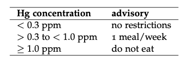
The RAFT program\(^{9}\) (Regional Ambient Fish Tissue) is an EPA effort to monitor concentrations of several harmful toxic substances in fish in the state of Iowa. This problem concerns the (slightly idealized and modified) values of mercury (chemical symbol Hg) detected in smallmounth bass sampled from two locations in Iowa. Samples of fish tissue were obtained as "plugs", taken from live fish in a manner similar to a biopsy. Typical plug samples weigh 50 mg. The criteria for issuing fish consumption advisories are shown in the table below. Plugs from smallmouth bass in Lake Wapello, IA contained on average 0.06 μg of Hg, while plugs from smallies in the Maquoketa River contained 0.01 μg Hg. Should there be consumption advisories for either waterbody?

Element 9.

\(^{9}\)Find more information about the EPA RAFT program by searching EPA raft on the web.

Chart

A simple solution method

Heuristic

Convert to uniform system of units

A useful first step is to identify the desired result. We’d like to find a Hg concentration in each fish in the same units that the advisory guidelines use: parts per million or ppm. This is a normalized and dimensionless, derived quantity. A second helpful step is therefore to express the key data in uniform units so that we can normalize them in dimensionless form. Our Hg measurements are in μg, which is 10\(^{−6}\) g, while our plug mass is in mg, which is 10\(^{−3}\) g. It doesn’t really matter whether we convert everything to grams or something else, but grams is straightforward. So now me construct the ratio that expresses how much mercury there is, by mass, in our fish tissue sample (using Lake Wapello values as an example):

\(\frac{0.06 x 10^{-6} g}{50 x 10^{-3} g}\) (5.8)

Simplify this by cancelling units and expressing each quantity in proper scientific notation:

\(\frac{6.0 x 10^{-8}}{5.0 x 10^{-2}}\) (5.9)

Using rules for division in exponents with a common base, we can simplify this:

\(\frac{6.0}{5.0}\) x 10\(^{(-8) - (-2)}\) (5.10)

The exponent therefore becomes −6, which you recall is the base for a “parts per million” ratio. We can simplify the fraction 6/5 either directly on a calculator, in our heads\(^{10}\), or by multiplying both numerator and denominator by two(= 12/10) and dividing by 10 to get 1.2:

6/5 × 10\(^{−6}\) = 1.2 ppm (5.11)

So the result for Wapello is 1.2 ppm, which exceeds safe limits for consumption. For the Maquoketa River, the Hg concentraion is only 0.2, so it is safe to eat and no advisory need be issued.

Element 10.

\(^{10}\)One great benefit of using scientific notation is that computations can be approximated easily by hand!

5.3.2 Example: forest fire losses (Problem 3.5)

Heuristic

Not enough information given? Make and state explicitly a reasonable and potentially-scalable assumption. If appropriate, choose values that can easily be scaled, like 1 or 10.

Let’s use some of the above techniques and strategies to make some ballpark estimates about the value of timber that could potentially be lost in a forest fire, following the teaser problem in Section 3.5. This could give us at least a starting point for imagining where the curve NVC starts from on the left-hand side of Figure 3.2. Since no specific information is given about the size of the property, we need to make and explicitly state an assumption. Let’s suppose for now that the property has an area of 1000 hectares, since that number is both reasonable for a single-ownership land parcel (this would be a bit less than 4 square miles) and is easily scaled. Let’s also assume that this 10 One great benefit of using scientific notation is that computations can be approximated easily by hand! forest in the absence of any fuel reduction effort is overstocked, with perhaps 30 m\(^{2}\) ha \(^{-1}\) of basal area\(^{11}\).

Element 11.

\(^{11}\)basal area, usually given in ft\(^{2}\) ac\(^{-1}\) (square feet per acre) or m\(^{2}\) ha\(^{−1}\) (square meters per hectare), provides a quick glimpse of the amount of standing timber on an area of land.

Using timber crushing charts, this basal area would yield about 30,000 board feet per hectare\(^{12}\). To get a ballpark estimate of the value of this timber then, we need to find the going price per board-foot of our timber and then scale this up with the timber volume and property area. A reasonable guess for the price for softwood saw-logs would be 0.20 US dollars (USD) per board foot\(^{13}\). So our computation becomes

NVC(0) = 1000 ha × 30000 BF/ha × 0.20 USD/BF.

Element 12.

\(^{12}\)One board-foot is equal to about 0.00236 m\(^{3}\) of wood.

Element 13.

\(^{13}\)A web search for “sawlog prices” can give you some idea of how this varies by place and time.

We can do this computation relatively quickly in a calculator, but there is a risk of typing in the wrong number of zeros and making an important error. However, if we convert these quantities to scientific notation and rewrite the equation we can do the math in our heads. The parcel area is 1 × 10\(^{3}\) hectares, the wood volume is 3 × 10\(^{4}\) board feet per hectare, and the value is 2 × 10\(^{−1}\) USD per board foot. So we may re-write the computation as

NVC(0) = 1×10\(^{3}\) ha × 3 × 10\(^{4}\) BF/ha × 2 × 10\(^{−1}\) USD/BF.

Since all these quantities are multiplied together, we can rearrange (by the commutative principle for multiplication) and group the mantissas together, put the powers together, and put the units together.

NVC(0) = 1 × 3 × 2 × 10\(^{3}\) × 10\(^{4}\) × 10\(^{−1}\) ha BF/ha USD/BF.

Multiplying the mantissas through we get 6, and using the rules for manipulating exponents (see the next section!) the exponents are added together (3 + 4 + −1) = 6. Canceling units, we see that USD is the only remaining unit. So our ballpark solution is that the value of the standing timber in this 1000 ha parcel is 6 × 10\(^{6}\) USD, or about $6 million.

Exercise 1

1. The Hg concentrations measured in the RAFT program problem were taken from “keeper” size smallmouth bass, roughly 35 cm long. A few scattered measurements from larger and smaller bass indicated that there was some systematic relationship between Hg concentrations and fish size at each site, but not across sites. What systematic relationships would you predict to be present in fish of different sizes? What quantities might be relevant to this problem? Formulate a testable hypothesis for expected systematic variation in smallmouth bass tissue Hg concentration as a function of fish size.

Exercise 2

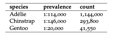
2. \(^{14}\)Leucism is partial albinism, manifested in penguins as a lack of (or substantial reduction in) pigment in plumage. A study of three species of penguin (Adélie, Gentoo and Chinstrap) in the Antarcic peninsula sought to identify the prevalence of leucism in these different species. The paper cited in the margin provides the following information derived from detailed counts of penguin breeding colonies made during the years 1994-1997:

Perform the following manipulations of the prevalence data for each species:

(a) Express the prevalence as a fraction (a ratio of whole numbers).

(b) Convert the prevalence to a decimal number.

(c) Convert the decimal number to scientific notation.

(d) Express the prevalence as a percentage of the population.

(e) Express the prevalence in parts per million (ppm).

(f) Determine the number of leucistic penguins in each count.

Element 14.

\(^{14}\)Based on the article ”Prevalence of leucism in Pygocelid penguins of the Antarctic Peninsula” by Forrest and Naveen, Waterbirds 23(2): 283-285, 2000.

Chart

Exercise 3

3. From our discussion of standing timber values (Section 5.3.2), how would the result be different if we learned that the land parcel was 385 hectares instead of 1000?