5.4: Graphical linear algebra

In this section we will begin to develop something called graphical linear algebra, which extends the ideas above. This formalism is actually quite powerful. For example, with it we can easily and graphically prove certain conjectures from control theory that, although they were eventually solved, required fairly elaborate matrix algebra arguments [FSR16].

presentation of Mat(R)

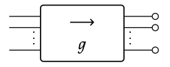
Let R be a rig, as defined in Definition 5.36. The main theorem of the previous section, Theorem 5.53, provided a functor S: SFG\(_{R}\) → Mat(R) that converts any signal flow

graph into a matrix. Next we show that S is “full”: that any matrix can be represented by a signal flow graph.

Proposition 5.56.

Given any matrix M \(\in\) Mat(R), there exists a signal flow graph g \(\in\) SFG\(_{R}\) such that such that S(g) = M.

Proof sketch. Let M \(\in\) Mat(R) be an (m × n)-matrix. We want a signal flow graph g such that S(g) = M. In particular, to compute S(g)(i, j), we know that we can simply compute the amplification that the i th input contributes to the j th output. The key idea then is to construct g so that there is exactly one path from i th input to the j th output, and that this path has exactly one scalar multiplication icon, namely M(i, j).

The general construction is a little technical (see Exercise 5.59), but the idea is clear from just considering the case of 2 × 2-matrices.

Suppose M is the 2 × 2-matrix \(\left(\begin{array}{ll} a & b \\ c & d \end{array}\right) .\) Then we define g to be the signal flow graph

Tracing paths, it is easy to see that S(g) = M. Note that g is the composite of four layers, each layer respectively a monoidal product of (i) copy and discard maps, (ii) scalar multiplications, (iii) swaps and identities, (iv) addition and zero maps. For the general case, see Exercise 5.59. \(\square\)

Exercise 5.58.

Draw signal flow graphs that represent the following matrices:

Exercise 5.59.

Write down a detailed proof of Proposition 5.56. Suppose M is an m × n-matrix. Follow the idea of the (2 × 2)-case in Eq. (5.57), and construct the signal flow graph g having m inputs and n outputs as the composite of four layers, respectively comprising (i) copy and discard maps, (ii) scalars, (iii) swaps and identities, (iv) addition and zero maps. ♦

We can also use Proposition 5.56 and its proof to give a presentation of Mat(R), which was defined in Definition 5.50.

Theorem 5.60.

The prop Mat(R) is isomorphic to the prop with the following presentation. The set of generators is the set

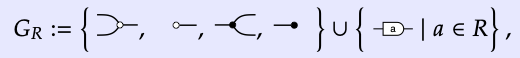
he same as the set of generators for SFGR; see Definition 5.45. We have the following equations for any a, b ∈ R:

Proof. The key idea is that these equations are sufficient to rewrite any GR-generated prop expression into a normal form—the one used in the proof of Proposition 5.56— with all the black nodes to the left, all the white nodes to the right, and all the scalars in the middle. This is enough to show the equality of any two expressions that represent the same matrix. Details can be found in [BE15] or [BS17] \(\square\)

Sound and complete presentation of matrices. Once you get used to it, Theorem 5.60 provides an intuitive, visual way to reason about matrices. Indeed, the theorem implies two signal flow graphs represent the same matrix if and only if one can be turned into the other by local application of the above equations and the prop axioms.

The fact that you can prove two SFGs to be the same by using only graphical rules can be stated in the jargon of logic: we say that the graphical rules provide a sound and complete reasoning system. To be more specific, sound refers to the forward direction of the above statement: two signal flow graphs represent the same matrix if one can be turned into the other using the given rules. Complete refers to the reverse direction: if two signal flow graphs represent the same matrix, then we can convert one into the other using the equations of Theorem 5.60.

Example 5.61.

Both of the signal flow graphs below represent the same matrix, \(\left(\begin{array}{l} 0 \\ 6 \end{array}\right):\)

This means that one can be transformed into the other by using only the equations from Theorem 5.60. Indeed, here

Exercise 5.62.

1. For each matrix in Exercise 5.58, draw another signal flow graph that represents that matrix.
2. Using the above equations and the prop axioms, prove that the two signal flow graphs represent the same matrix. ♦

Exercise 5.63.

Consider the signal flow graphs

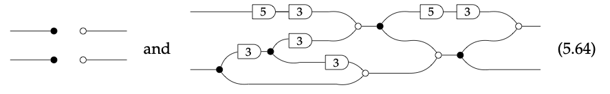
1. Let R = (\(\mathbb{N}\), 0, +, 1, ∗). By examining the presentation of Mat(R) in Theorem 5.60, and without computing the matrices that the two signal flow graphs in Eq. (5.64) represent, prove that they do not represent the same matrix.
2. Now suppose the rig is R = \(\mathbb{N}\)/3\(\mathbb{N}\); if you do not know what this means, just replace all 3’s with 0’s in the right-hand diagram of Eq. (5.64). Find what you would call a minimal representation of this diagram, using the presentation in Theorem 5.60. ♦

Aside: monoid objects in a monoidal category

Various subsets of the equations in Theorem 5.60 encode structures that are familiar from many other parts of mathematics, e.g. representation theory. For example one can find the axioms for (co)monoids, (co)monoid homomorphisms, Frobenius algebras, and (with a little rearranging) Hopf algebras, sitting inside this collection. The first example, the notion of monoids, is particularly familiar to us by now, so we briefly discuss it below, both in algebraic terms (Definition 5.65) and in diagrammatic terms (Example 5.68).

Definition 5.65.

A monoid object (M, μ, η) in a symmetric monoidal category (C, I, ⊗) is an object M of C together with morphisms μ: M ⊗ M → M and η: I → M such that

(a) (μ ⊗ id) ; μ = (id ⊗ μ) ; μ and

(b) (η ⊗ id) ; μ = id = (id ⊗ η) ; μ.
A commutative monoid object is a monoid object that further obeys

(c) σ\(_{M,M}\) ; μ = μ.
where σ\(_{M,M}\) is the swap map on M in C. We often denote it simply by σ.

Monoid objects are so-named because they are an abstraction of the usual concept of monoid.

Example 5.66.

A monoid object in (Set, 1, ×) is just a regular old monoid, as defined in Example 2.6; see also Example 3.13.

That is, it is a set M, a function μ: M × M → M, which we denote by infix notation ∗, and an element η(1) \(\in\) M, which we denote by e, satisfying (a ∗ b) ∗ c = a ∗ (b ∗ c) and a ∗ e = a = e ∗ a.

Exercise 5.67.

Consider the set \(\mathbb{R}\) of real numbers.

1. Show that if μ: \(\mathbb{R}\) × \(\mathbb{R}\) → \(\mathbb{R}\) is defined by μ(a, b) = a ∗ b and if η \(\in\) \(\mathbb{R}\) is defined to be η = 1, then (\(\mathbb{R}\), ∗, 1) satisfies all three conditions of Definition 5.65.
2. Show that if μ: \(\mathbb{R}\) × \(\mathbb{R}\) → \(\mathbb{R}\) is defined by μ(a,b) = a + b and if η \(\in\) \(\mathbb{R}\) is defined to be η = 0, then (\(\mathbb{R}\), +, 0) satisfies all three conditions of Definition 5.65. ♦

Example 5.68.

Graphically, we can depict . Then axioms (a), (b), and (c) from Definition 5.65 become:

All three of these are found in Theorem 5.60. Thus we can immediately conclude the following: the triple is a commutative monoid object in the prop Mat(R).

Exercise 5.69.

For any rig R, there is a functor U : Mat(R) → Set, sending the object n \(\in\) \(\mathbb{N}\) to the set R\(^{n}\), and sending a morphism (matrix) M: m → n to the function R\(^{m}\) → R\(^{n}\) given by vector-matrix multiplication.

Recall that in Mat(R), the monoidal unit is 0 and the monoidal product is +, because it is a prop. Recall also that in (the usual monoidal structure on) Set, the monoidal unit is {1}, a set with one element, and the monoidal product is × (see Example 4.49).

1. Check that the functor U : Mat(R) → Set, defined above, preserves the monoidal unit and the monoidal product.
2. Show that if (M, μ, η) is a monoid object in Mat(R) then (U(M), U(μ), U(η)) is a monoid object in Set. (This works for any monoidal functor—which we will define in Definition 6.68—not just for U in particular.)
3. In Example5.68, we said that the triple is a commutative monoid object in the prop Mat(R). If R = \(\mathbb{R}\) is the rig of real numbers, this means that we have a monoid structure on the set \(\mathbb{R}\). But in Exercise 5.67 we gave two such monoid structures. Which one is it? ♦

Example 5.70.

The triple in Mat(R) forms a commutative monoid object in Mat(R)op. We hence also say that forms a co-commutative comonoid object in Mat(R).

Example 5.71.

A symmetric strict monoidal category, is just a commutative monoid object in (Cat, ×, 1). We will unpack this in Section 6.4.1.

Example 5.72.

A symmetric monoidal preorder, which we defined in Definition 2.2, is just a commutative monoid object in the symmetric monoidal category (Preord, ×, 1) of preorders and monotone maps.

Example 5.73.

For those who know what tensor products of commutative monoids are (or can guess): A rig is a monoid object in the symmetric monoidal category (CMon, ⊗, \(\mathbb{N}\)) of commutative monoids with tensor product.

Remark 5.74. If we present a prop M using two generators μ: 2 → 1 and η: 0 → 1, and the three equations from Definition 5.65, we could call it ‘the theory of monoids in monoidal categories.’ This means that in any monoidal category C, the monoid objects in C correspond to strict monoidal functors M → C. This sort of idea leads to the study of algebraic theories, due to Bill Lawvere and extended by many others; see Section 5.5.

Signal flow graphs: feedback and more

At this point in the story, we have seen that every signal flow graph represents a matrix, and this gives us a new way of reasoning about matrices. This is just the beginning of a beautiful tale, one not only of graphical matrices, but of graphical linear algebra. We close this chapter with some brief hints at how the story continues.

The pictoral nature of signal flow graphs invites us to play with them. While we normally draw the copy icon like so,, we could just as easily reverse it and draw an icon . What might it mean? Let’s think again about the semantics of flow graphs.

The behavioral approach. A signal flow graph g : m → n takes an input x \(\in\) R\(^{m}\) and gives an output y \(\in\) R\(^{n}\). In fact, since this is all we care about, we might just think about representing a signal flow graph g as describing a set of input and output pairs (x, y).

We’ll call this set the behavior of g and denote it B(g) \(\subseteq\) R\(^{m}\) × R\(^{n}\). For example, the ‘copy’ flow graph

sends the input 1 to the output (1, 1), so we consider (1, (1, 1)) to be an element of copy-behavior. Similarly, (x, (x, x)) is copy behavior for every x \(\in\) R, thus we have

In the abstract, the signal flow graph g : m → n has the behavior

\(\mathrm{B}(g)=\left\{(x, S(g)(x)) \mid x \in R^{m}\right\} \subseteq R^{m} \times R^{n}\) (5.75)

Mirror image of an icon. The above behavioral perspective provides a clue about how to interpret the mirror images of the diagrams discussed above.

Reversing an icon g: m → n exchanges the inputs with the outputs, so if we denote this reversed icon by g\(^{op}\), we must have g\(^{op}\): n → m. Thus if B(g) \(\subseteq\) R\(^{m}\) × R\(^{n}\) then we need B(g\(^{op}\)) \(\subseteq\) R\(^{m}\) × R\(^{n}\). One simple way to do this is to replace each (a, b) with (b, a), so we would have

\(\begin{equation}
\mathrm{B}\left(g^{\mathrm{op}}\right):=\left\{(S(g)(x), x) \mid x \in R^{m}\right\} \subseteq R^{n} \times R^{m}
\end{equation}\) (5.76)

This is called the transposed relation.

Exercise 5.77.

1. What is the behavior B() of the reversed addition icon : 1→ 2?

2. What is the behavior B() of the reversed copy icon, : 2→ 1? ♦

Eqs. (5.75) and (5.76) give us formulas for interpreting signal flow graphs and their mirror images. But this would easily lead to disappointment, if we couldn’t combine the two directions behaviorally; luckily we can.

Combining directions. What should the behavior be for a diagram such as the following:

Let’s formalize our thoughts a bit and begin by thinking about behaviors. The behavior of a signal flow graph m → n is a subset B \(\subseteq\) R\(^{m}\) × R\(^{n}\), i.e. a relation. Why not try to construct a prop where the morphisms m → n are relations?

We’ll need to know how to compose and take monoidal products of relations. And if we want this prop of relations to contain the old prop Mat(R), we need the new compositions and monoidal products to generalize the old ones in Mat(R). Given signal flow graphs with matrices M: m → n and N: n → p, we see that their behaviors are the relations \(B_{1}\) := {(x,Mx) | x \(\in\) \(R^{m}\)} and \(B_{2}\) := {(y, Ny) | y \(\in\) \(R^{n}\), while the behavior of M ; N is the relation {(x, x ; M ; N) | x \(\in\) \(R^{m}\)}. This is a case of relation composition. Given relations \(B_{1}\) \(\subseteq\) R\(^{m}\) × R\(^{n}\) and \(B_{2}\) \(\subseteq\) R\(^{n}\) × R\(^{p}\), their composite \(B_{1}\) ; \(B_{2}\) \(\subseteq\) R\(^{m}\) × R\(^{p}\)is given by

\(B_{1} \text { ; } B_{2}:=\left\{(x, z) \mid \text { there exists } y \in R^{n} \text { such that }(x, y) \in B_{1} \text { and }(y, z) \in B_{2}\right\}\) (5.78)

We shall use this as the general definition for composing two behaviors.

Definition 5.79.

Let R be a rig. We define the prop Rel\(_{R}\) of R-relations to have subsets B \(\subseteq\) R\(^{m}\) × R\(^{n}\) as morphisms. These are composed by the composition rule from Eq. (5.78), and we take the product of two sets to form their monoidal product.

Exercise 5.80.

In Definition 5.79 we went quickly through monoidal products + in the prop Rel\(_{R}\). If B \(\subseteq\) R\(^{m}\) × R\(^{n}\) and C \(\subseteq\) R\(^{n}\) × R\(^{p}\) are morphisms in Rel\(_{R}\), write down B + C in set-notation. ♦

(No-longer simplified) signal flow graphs. Recall that above, e.g. in Definition 5.45, we wrote GR for the set of generators of signal flow graphs. In Section 5.4.3, we wrote g\(^{op}\) for the mirror image of g, for each g \(\in\) G\(_{R}\). So let’s write G\(_{R}\) := {g\(^{op}\) | g \(\in\) G\(_{R}\)} for the set of all the mirror images of generators. We define a prop

\(\mathbf{S F G}_{R}^{+}:=\text {Free }\left(G_{R} \sqcup G_{R}^{\mathrm{op}}\right)\) (5.81)

We call a morphism in the prop \(\mathbf{S F G}_{R}^{+}\) a a (non-simplified) signal flow graph: these extend our simplified signal flow graphs from Definition 5.45 because now we can also use the mirrored icons. By the universal property of free props, since we have said what the behavior of the generators is (the behavior of a reversed icon is the transposed relation; see Eq. (5.76)), we have specified the behavior of any signal flow graph. The following two exercises help us understand what this behavior is.

Exercise 5.82.

Let g :m → n, h :l → n be signal flow graphs. Note that h\(^{op}\) :n → l is a signal flow graph, and we can form the composite g ; (h\(^{op}\)):

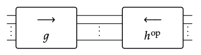
Show that the behavior of g ; (h\(^{op}\)) \(\subseteq\) R\(^{m}\) × R\(^{l}\) is equal to

\(\mathrm{B}\left(g \text { ; }\left(h^{\mathrm{op}}\right)\right)=\{(x, y) \mid S(g)(x)=S(h)(y)\}\) ♦

Exercise 5.83.

Let g :m → n, h : m → p be signal flow graphs. Note that (g\(^{op}\)) : n → m is a signal flow graph, and we can form the composite g\(^{op}\) ; h

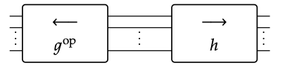
Show that the behavior of g\(^{op}\) ; h is equal to

\(\mathrm{B}\left(\left(g^{\mathrm{op}}\right) ; h\right)=\left\{(S(g)(x), S(h)(x)) \mid x \in R^{m}\right\}\) ♦

Linear algebra via signal flow graphs. In Eq. (5.75) we see that every matrix, or linear map, can be represented as the behavior of a signal flow graph, and in Exercise 5.82 we see that solution sets of linear equations can also be represented. This includes central concepts in linear algebra, like kernels and images.

Exercise 5.84.

Here is an exercise for those that know linear algebra, in particular kernels and cokernels.

Let R be a field, let g : m → n be a signal flow graph, and let S(g) \(\in\) Mat(R) be the associated (m × n) matrix (see Theorem 5.53).

1. Show that the composite of g with 0-reverses, shown here

is equal to the kernel of the matrix S(g).

2. Show that the composite of discard-reverses with g, shown here

is equal to the image of the matrix S(g).

3. Show that for any signal flow graph g, the subset B(g) \(\subseteq\) R\(^{m}\) × R\(^{n}\) is a linear subspace.

That is, if b\(_{1}\), b\(_{2}\) \(\in\) B(g) then so are b\(_{1}\) + b\(_{2}\) and r ∗ b\(_{1}\), for any r \(\in\) R. ♦

We have thus seen that signal flow graphs provide a uniform, compositional language to talk about many concepts in linear algebra. Moreover, in Exercise 5.84 we showed that the behavior of a signal flow graph is a linear relation, i.e. a relation whose elements can be added and multiplied by scalars r \(\in\) R. In fact the converse is true too: any linear relation B \(\subseteq\) R\(^{m}\) × R\(^{n}\) can be represented by a signal flow graph.

Exercise 5.85.

One might want to show that linear relations on R form a prop, LinRel\(_{R}\) . That is, one might want to show that there is a sub-prop of the prop Rel\(_{R}\) from Definition 5.79, where the morphisms m → n are the subsets B \(\subseteq\) R\(^{m}\) × R\(^{n}\) such that B is linear.

In other words, where for any (x, y) \(\in\) B and r \(\in\) R, the element (r ∗ x, r ∗ y) \(\in\) R\(^{m}\) × R\(^{n}\) is in B, and for any (x′, y′) \(\in\) B, the element (x + x′, y + y′) is in B.

This is certainly doable, but for this exercise, we only ask that you prove that the composite of two linear relations is linear. ♦

Just like we gave a sound and complete presentation for the prop of matrices in Theorem 5.60, it is possible to give a sound and complete presentation for linear relations on R. Moreover, it is possible to give such a presentation whose generating op

set is GR ⊔ GR as in Eq. (5.81) and whose equations include those from Theorem 5.60, plus a few more. This presentation gives a graphical method for doing linear algebra: an equation between linear subspaces is true if and only if it can be proved using the equations from the presentation.

Although not difficult, we leave the full presentation to further reading (Section 5.5). Instead, we’ll conclude our exploration of the prop of linear relations by noting that some of these ‘few more’ equations state that relations just like co-design problems in Chapter 4 form a compact closed category.

Compact closed structure. Using the icons available to us for signal flow graphs, we can build morphisms that look like the ‘cup’ and ‘cap’ from Definition 4.58:

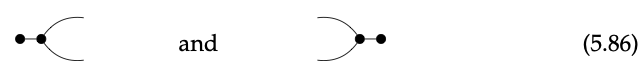
The behaviors of these graphs are respectively

\(\{(0,(x, x)) \mid x \in R\} \subseteq R^{0} \times R^{2} \quad \text { and } \quad\{((x, x), 0) \mid x \in R\} \subseteq R^{2} \times R^{0}\)

In fact, these show the object 1 in the prop Rel\(_{R}\) is dual to itself: the morphisms from Eq. (5.86) serve as the η\(_{1}\) and ε\(_{1}\) from Definition 4.58. Using monoidal products of these morphisms, one can show that any object in Rel\(_{R}\) is dual to itself.

Graphically, this means that the three signal flow graphs

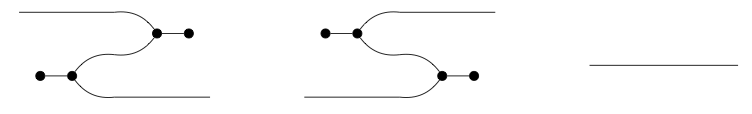
all represent the same relation.
Using these relations, it is straightforward to check the following result.

Theorm 5.87.

The prop Rel\(_{R}\) is a compact closed category in which every object n \(\in\) \(\mathbb{N}\) is dual to itself, n = n\(^{∗}\).

To make our signal flow graphs simpler, we define new icons cup and cap by the equations

Back to control theory. Let’s close by thinking about how to represent a simple control theory problem in this setting. Suppose we want to design a system to maintain the speed of a car at a desired speed u. We’ll work in signal flow diagrams over the rig \(\mathbb{R}\)[s, s\(^{−1}\)] of polynomials in s and s\(^{−1}\) with coefficients in \(\mathbb{R}\) and where ss\(^{−1}\) = s\(^{−1}\)s = 1. This is standard in control theory: we think of s as integration, and s\(^{−1}\) as differentiation.

There are three factors that contribute to the actual speed v. First, there is the actual speed v. Second, there are external forces F. Third, we have our control system: this will take some linear combination a ∗ u + b ∗ v of the desired speed and actual speed, amplify it by some factor p to give a (possibly negative) acceleration. We can represent this system as follows, where m is the mass of the car.

This can be read as the following equation, where one notes that v occurs twice:

\(v=\int \frac{1}{m} F(t) d t+u(t)+p \int a u(t)+b v(t) d t\)

Our control problem then asks: how do we choose a and b to make the behavior of this signal flow graph close to the relation {(F, u, v) | u = v}? By phrasing problems in this way, we can use extensions of the logic we have discussed above to reason about such complex, real-world problems.