6.1: The ubiquity of network languages

Electric circuits, chemical reaction networks, finite state automata, Markov processes: these are all models of physical or computational systems that are commonly described using network diagrams. Here, for example, we draw a diagram that models a flip-flop, an electric circuit important in computer memory that can store a bit of information:

Network diagrams have time-tested utility. In this chapter, we are interested in understanding the common mathematical structure that they share, for the purposes of translating between and unifying them; for example certain types of Markov processes can be simulated and hence solved using circuits of resisters. When we understand the underlying structures that are shared by network diagram languages, we can make comparisons between the corresponding mathematical models easily.

At first glance network diagrams appear quite different from the wiring diagrams we have seen so far. For example, the wires are undirected in the case above, whereas in a category including monoidal categories seen in resource theories or co-design every morphism has a domain and codomain, giving it a sense of direction. Nonetheless, we shall see how to use categorical constructions such as universal properties to create categorical models that precisely capture the above type of “network” compositionality, i.e. allowing us to effectively drop directedness when convenient.

In particular we’ll return to the idea of a colimit, which we sketched for you at the end of Chapter 3, and show how to use colimits in the category of sets to formalize ideas of connection. Here’s the key idea.

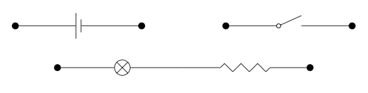
Connections via colimits. Let’s say we want to install some lights: we want to create a circuit so that when we flick a switch, a light turns on or off. To start, we have a bunch of circuit components: a power source, a switch, and a lamp connected to a resistor:

We want to connect them together, but there are many ways to do so. How should we describe the particular way that will form a light switch?

First, we claim that circuits should really be thought of as open circuits: each carries the additional structure of an ‘interface’ exposing it to the rest of the electrical world. Here by interface we mean a certain set of locations, or ports, at which we are able to connect them with other components.1 As is so common in category theory, we begin by making this more-or-less obvious fact explicit. Let’s depict the available ports using a bold •. If we say that in the each of the three drawings above, the ports are simply the dangling end points of the wires, they would be redrawn as follows:

Next, we have to describe which ports should be connected. We’ll do this by draw- ing empty circles ◦ connected by arrows to two ports •. Each will be a witness-to- connection, saying ‘connect these two!’

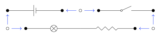
Looking at this picture, it is clear what we need to do: just identify—i.e. merge or make equal—the ports as indicated, to get the following circuit:

But mathematics doesn’t have a visual cortex with which to generate the intuitions we can count on with a human reader such as yourself.\(^{2}\) Thus we need to specify formally what ‘identifying ports as indicated’ means mathematically. As it turns out, we can do this using finite colimits in a given category C.

Colimits are diagrams with certain universal properties, which is kind of an epiphe- nomenon of the category C. Our goal is to obtain C’s colimits more directly, as a kind of operation in some context, so that we can think of them as telling us how to connect circuit parts together. To that end, we produce a certain monoidal category namely that of cospans in C, denoted Cospan\(_{C}\) that can conveniently package C’s colimits in terms of its own basic operations: composition and monoidal product.

In summary, the first part of this chapter is devoted to the slogan ‘colimits model interconnection’. In addition to universal constructions such as colimits, however, another way to describe interconnection is to use wiring diagrams. We go full circle when we find that these wiring diagrams are strongly connected to cospans, and hence colimits.

But mathematics doesn’t have a visual cortex with which to generate the intuitions we can count on with a human reader such as yourself.2 Thus we need to specify formally what ‘identifying ports as indicated’ means mathematically. As it turns out, we can do this using finite colimits in a given category C.

Colimits are diagrams with certain universal properties, which is kind of an epiphe- nomenon of the category C. Our goal is to obtain C’s colimits more directly, as a kind of operation in some context, so that we can think of them as telling us how to connect circuit parts together. To that end, we produce a certain monoidal category namely that of cospans in C, denoted Cospan\(_{C}\) that can conveniently package C’s colimits in terms of its own basic operations: composition and monoidal product.

In summary, the first part of this chapter is devoted to the slogan ‘colimits model interconnection’. In addition to universal constructions such as colimits, however, another way to describe interconnection is to use wiring diagrams. We go full circle when we find that these wiring diagrams are strongly connected to cospans, and hence colimits.

Composition operations and wiring diagrams. In this book we have seen the utility of defining syntactic or algebraic structures that describe the sort of composition op- erations that make sense and can be performed in a given application area. Examples include monoidal preorders with discarding, props, and compact closed categories. Each of these has an associated sort of wiring diagram style, so that any wiring dia- gram of that style represents a composition operation that makes sense in the given area: the first makes sense in manufacturing, the second in signal flow, and the third in collaborative design. So our second goal is to answer the question, “how do we describe the compositional structure of network-style wiring diagrams?”

Network-type interconnection can be described using something called a hyper- graph category. Roughly speaking, these are categories whose wiring diagrams are those of symmetric monoidal categories together with, for each pair of natural numbers (m, n), an icon s\(_{m,n}\) : m → n. These icons, known as spiders,\(^{3}\) are drawn as follows:

Two spiders can share a leg, and when they do, we can fuse them into one spider. The intuition is that spiders are connection points for a number of wires, and when two connection points are connected, they fuse to form an even more ‘connect-y’ connection point. Here is an example:

A hypergraph category may have many species of spiders with the rule that spiders of different species cannot share a leg and hence not fuse but two spiders of the same species can share legs and fuse. We add spider diagrams to the iconography of hypergraph categories.

As we shall see, the ideas of describing network interconnection using colimits and hypergraph categories come together in the notion of a theory. We first introduced the idea of a theory in Section 5.4.2, but here we explore it more thoroughly, starting with the idea that, approximately speaking, cospans in the category FinSet form the theory of hypergraph categories.

We can assemble all cospans in FinSet into something called an ‘operad’. Through- out this book we have talked about using free structures and presentations to create instances of algebraic structures such as preorders, categories, and props, tailored to the needs of a particular situation. Operads can be used to tailor the algebraic structures themselves to the needs of a particular situation. We will discuss how this works, in particular how operads encode various sorts of wiring diagram languages and corresponding algebraic structures, at the end of the chapter.