6.2: Colimits and Connection

Universal constructions are central to category theory. They allow us to define objects, at least up to isomorphism, by describing their relationship with other objects. So far we have seen this theme in a number of different forms: meets and joins (Section 1.3), Galois connections and adjunctions (Sections 1.4 and 3.4), limits (Section 3.5), and free and presented structures (Section 5.2.3-5.2.5). Here we turn our attention to colimits.

In this section, our main task is to have a concrete understanding of colimits in the category FinSet of finite sets and functions. The idea will be to take a bunch of sets say two or fifteen or zero use functions between them to designate that elements in one set ‘should be considered the same’ as elements in another set, and then merge the sets together accordingly.

Initial objects

Just as the simplest limit is a terminal object (see Section 3.5.1), the simplest colimit is an initial object. This is the case where you start with no objects and you merge them together.

Definition 6.1.

Let C be a category. An initial object in C is an object Ø \(\in\) C such that for each object T in C there exists a unique morphism !\(_{T}\) : Ø → T.

The symbol Ø is just a default name, a notation, intended to evoke the right idea; see Example 6.4 for the reason why we use the notation Ø, and Exercise 6.7 for a case when the default name Ø would probably not be used.

Again, the hallmark of universality is the existence of a unique map to any other comparable object.

Example 6.2.

An initial object of a preorder is a bottom element that is, an element that is less than every other element.

For example 0 is the initial object in (\(\mathbb{N}\), ≤), whereas (\(\mathbb{R}\), ≤) has no initial object.

Exercise 6.3.

Consider the set A = {a, b}. Find a preorder relation ≤ on A such that

1. (A, ≤) has no initial object.

2. (A, ≤) has exactly one initial object.

3. (A, ≤) has two initial objects. ♦

Example 6.4.

The initial object in FinSet is the empty set. Given any finite set T, there is a unique function Ø → T, since Ø has no elements.

Example 6.5.

As seen in Exercise 6.3, a category C need not have an initial object. As a different sort of example, consider the category shown here:

If there were to be an initial object Ø, it would either be A or B.

Either way, we need to show that for each object T \(\in\) Ob(C) (i.e. for both T = A and T = B) there is a unique morphism Ø → T. Trying the case Ø =\(^{?}\) A this condition fails when T = B: there are two morphisms A → B, not one.

And trying the case Ø =\(^{?}\) B this condition fails when T = A: there are zero morphisms B → A, not one.

Exercise 6.6.

For each of the graphs below, consider the free category on that graph, and say whether it has an initial object.

Exercise 6.7.

Recall the notion of rig from Chapter 5.

A rig homomorphism from (R, 0\(_{R}\), +\(_{R}\), 1\(_{R}\), ∗\(_{R}\)) to (S, 0\(_{S}\), +\(_{S}\), 1\(_{S}\), ∗\(_{S}\)) is a function f : R → S such that f (0\(_{R}\)) = 0\(_{S}\), f (r1 +\(_{R}\) r2) = f (r1) +\(_{S}\) f (r2),etc.

1. We said “etc.” Guess the remaining conditions for f to be a rig homomorphism.

2. Let Rig denote the category whose objects are rigs and whose morphisms are rig homomorphisms. We claim Rig has an initial object. What is it? ♦

Exercise 6.8.

Explain the statement “the hallmark of universality is the existence of a unique map to any other comparable object,” in the context of Definition 6.1. In particular, what is being universal in Definition 6.1, and which is the “comparable object”? ♦

Remark 6.9. As mentioned in Remark 3.85, we often speak of ‘the’ object that satisfies a universal property, such as ‘the initial object’, even though many different objects could satisfy the initial object condition. Again, the reason is that initial objects are unique up to unique isomorphism: any two initial objects will have a canonical isomorphism between them, which one finds using various applications of the universal property.

Exercise 6.10.

Let C be a category, and suppose that c\(_{1}\) and c\(_{2}\) are initial objects. Find an isomorphism between them, using the universal property from Definition 6.1. ♦

Coproducts

Coproducts generalize both joins in a preorder and disjoint unions of sets.

Definition 6.11.

Let A and B be objects in a category C.

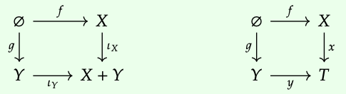
A coproduct of A and B is an object, which we denote A + B, together with a pair of morphisms (ι\(_{A}\) : A → A + B, ι\(_{B}\) : B → A + B) such that for all objects T and pairs of morphisms (f : A → T, g : B → T), there exists a unique morphism [f , g]: A + B → T such that the following diagram commutes:

We call [f , g] the copairing of f and g.

Exercise 6.13.

Explain why, in a preorder, coproducts are the same as joins. ♦

Example 6.14.

Coproducts in the categories FinSet and Set are disjoint unions. More precisely, suppose A and B are sets.

Then the coproduct of A and B is given by the disjoint union A ⊔ B together with the inclusion functions ι\(_{A}\) : A → A ⊔ B and ι\(_{B}\) : B → A ⊔ B.

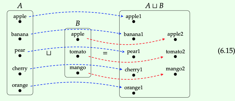
Suppose we have functions f: A → T and g: B → T for some other set T, unpictured. The universal property of coproducts says there is a unique function [ f , g] : A ⊔ B → T such that ι\(_{A}\) ; [ f , g] = f and ι\(_{B}\) ; [ f ,g ] = g.

What is it? Any element x \(\in\) A ⊔ B is either ‘from A’ or ‘from B’, i.e. either there is some a \(\in\) A with x = ι\(_{A}\)(a) or there is some b \(\in\) B with x = ι\(_{B}\)(b). By Eq. (6.12), we must have:

\([f, g](x)=\left\{\begin{array}{ll}
f(x) & \text { if } x=\iota_{A}(a) \text { for some } a \in A \\
g(x) & \text { if } x=\iota_{B}(b) \text { for some } b \in B
\end{array}\right.\)

Exercise 6.16.

Suppose T = {a, b, c, . . . , z} is the set of letters in the alphabet, and let A and B be the sets from Eq. (6.15). Consider the function f : A → T sending each element of A to the first letter of its label, e.g. f(apple) = a. Let g: B → T be the function sending each element of B to the last letter of its label, e.g. g(apple) = e. Write down the function [f , g](x) for all eight elements of A ⊔ B. ♦

Exercise 6.17.

Let f : A → C, g : B → C, and h :C → D be morphisms in a category C with coproducts. Show that

1. ι\(_{A}\) ; [f , g] = f .
2. ι\(_{B}\) ; [f, g] = g.
3. [f, g] ; h = [f ; h, g ; h].
4. [ι\(_{A}\), ι\(_{B}\)] = id\(_{A+B}\). ♦

Exercise 6.18.

Suppose a category C has coproducts, denoted +, and an initial object, denoted Ø. Then (C, +, Ø) is a symmetric monoidal category (recall Definition 4.45). In this exercise we develop the data relevant to this fact:

1. Show that + extends to a functor C × C → C. In particular, how does it act on morphisms in C × C?

2. Using the universal properties of the initial object and coproduct, show that there are isomorphisms A + Ø → A and Ø + A → A.

3. Using the universal property of the coproduct, write down morphisms

a) (A + B) + C → A + (B + C).

b) A + B → B + A.

If you like, check that these are isomorphisms.

It can then be checked that this data obeys the axioms of a symmetric monoidal category, but we’ll end the exercise here. ♦

Pushouts

Pushouts are a way of combining sets. Like a union of subsets, a pushout can combine two sets in a non-disjoint way: elements of one set may be identified with elements of the other. The pushout construction, however, is much more general: it allows (and requires) the user to specify exactly which elements will be identified. We’ll see a demonstration of this additional generality in Example 6.29

Definition 6.19.

Let C be a category and let f :A → X and g : A → Y be morphisms in C that have a common domain. The pushout X +\(_{A}\)Y is the colimit of the diagram

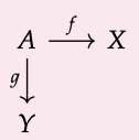
In more detail, a pushout consists of (i) an object X +\(_{A}\)Y and (ii) morphisms ι\(_{X}\) : X → X +\(_{A}\)Y and ι\(_{Y}\) : Y → X + \(_{A}\)Y satisfying (a) and (b) below.

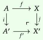
(a) The diagram

commutes. (We will explain the ‘\(\Gamma\)’ symbol below.)

(b) For all objects T and morphisms x: X → T, y: Y → T, if the diagram

commutes, then there exists a unique morphism t : X +\(_{A}\)Y → T such that

commutes.

If X + \(_{A}\)Y is a pushout, we denote that fact by drawing the commutative square Eq. (6.20), together with the \(\Gamma\) symbol as shown; we call it a pushout square. We further call ι\(_{X}\) the pushout of g along f , and similarly ι\(_{Y}\) the pushout of f along g.

Example 6.22.

In a preorder, pushouts and coproducts have a lot in common. The pushout of a diagram B ← A → C is equal to the coproduct B ⊔ C: namely, both are equal to the join B \(\bigvee\) C.

Example 6.23.

Let f : A → X be a morphism in a category C. For any isomorphisms i : A → A′ and j : X → X′, we can take X′ to be the pushout X + \(_{A}\) A′, i.e. the following is a pushout square:

where f' := i\(^{-1}\) ; f ; j. To see this, observe that if there is any object T such that the following square commutes:

then f ; x = i ; a, and so we are forced to take x': X → T to be x' := j\(^{-1}\) ; x. This makes the following diagram commute:

because f' ; x' = i\(^{-1}\) ; f ; j ; j\(^{-1}\) ; x = i\(^{-1}\) ; i ; a = a.

Exercise 6.24.

For any set S, we have the discrete category Disc\(_{S}\), with S as objects and only identity morphisms.

1. Show that all pushouts exist in Disc\(_{S}\), for any set S.
2. For what sets S does Disc\(_{S}\) have an initial object? ♦

Example 6.25.

In the category FinSet, pushouts always exist. The pushout of functions f : A → X and g : A → Y is the set of equivalence classes of X ⊔ Y under the equivalence relation generated by that is, the reflexive, transitive, symmetric closure of the relation {f(a) ∼ g(a) | a \(\in\) A}.
We can think of this in terms of interconnection too. Each element a \(\in\) A provides a connection between f (a) in X and g(a) in Y.

The pushout is the set of connected components of X ⊔ Y.

Exercise 6.26.

What is the pushout of the functions f : \(\underline{4}\) → \(\underline{5}\) and g : \(\underline{4}\) → \(\underline{3}\) pictured below?

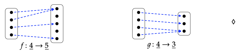
Check your answer using the abstract description from Example 6.25.

Example 6.27.

Suppose a category C has an initial object Ø. For any two objects X, Y \(\in\) ObC, there is a unique morphism f : Ø → X and a unique morphism g : Ø → Y; this is what it means for Ø to be initial.

The diagram \(X \stackrel{f}{\rightarrow} Ø \stackrel{g}{\leftarrow} Y\) has a pushout in C iff X andY have a coproduct in C, and the pushout and the coproduct will be the same. Indeed, suppose X and Y have a coproduct X + Y; then the diagram to the left

commutes (why?\(^{1}\)), and for any object T and commutative diagram as to the right, there is a unique map X + Y → T making the diagram as in Eq. (6.21) commute (why?\(^{2}\)). This shows that X + Y is a pushout, X + \(_{Ø}\)Y \(\cong\) X + Y.

Similarly, if a pushout X + Y exists, then it satisfies the universal property of the coproduct (why? \(^{3}\)).

Exercise 6.28.

In Example 6.27 we asked “why?” three times.

1. Give a justification for “why?\(^{1}\)”.

2. Give a justification for “why\(^{2}\)? ”.

3. Give a justification for “why?\(^{3}\)”. ♦

Example 6.29.

LetA = X = Y = N. Consider the functions f : A → X and g : A → Y given by the ‘floor’ functions, f (a) := ⌊a/2⌋ and g(a) := ⌊(a + 1)/2⌋.

What is their pushout? Let’s figure it out using the definition.

If T is any other set and we have maps x : X → T and y : Y → T that commute with f and g, i.e. f \(\cong\) x = g \(\cong\) y, then this commutativity implies that

y(0) = y(g(0)) = x(f (0)) = x(0).

In other words,Y ’s 0 and X ’s 0 go to the same place in T, say t. But since f(1) = 0 and g(1) = 1, we also have that t = x(0) = x(f(1)) = y(g(1)) = y(1). This means Y’s 1 goes to t also. But since g(2) = 1 and f (2) = 1, we also have that t = g(1) = y(g(2)) = x( f (2)) = x(1), which means that X’s 1 also goes to t. One can keep repeating this and find that every element of Y and every element of X go to t! Using mathematical induction, one can prove that the pushout is in fact a 1-element set, X ⊔A Y \(\cong\) {1}.

Finite colimits

Initial objects, coproducts, and pushouts are all types of colimits. We gave the general definition of colimit in Section 3.5.4. Just as a limit in C is a terminal object in a category of cones over a diagram D : J → C, a colimit is an initial object in a category of cocones over some diagram D : J → C. For our purposes it is enough to discuss finite colimits—i.e. when J is a finite category—which subsume initial objects, coproducts, and pushouts.\(^{4}\)

In Definition 3.102, cocones in C are defined to be cones in C\(^{op}\). For visualization purposes, if D : J → C looks like the diagram to the left, then a cocone on it shown in the diagram to the right:

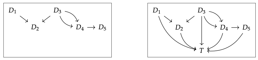
Here, any two parallel paths that end at T are equal in C.

Definition 6.30.

We say that a category C has finite colimits if a colimit, colim\(_{J}\) D, exists whenever J is a finite category and D : J → C is a diagram.

Example 6.31.

The initial object in a category C, if it exists, is the colimit of the functor ! : 0 → C, where 0 is the category with no objects and no morphisms, and ! is the unique such functor. Indeed, a cocone over ! is just an object of C, and so the initial cocone over ! is just the initial object of C.

Note that 0 has finitely many objects (none); thus initial objects are finite colimits.

We often want to know that a category C has all finite colimits (in which case, we often drop the ‘all’ and just say ‘C has finite colimits’). To check that C has (all) finite colimits, it’s enough to check it has a few simpler forms of colimit, which generate all the rest.

Proposition 6.32.

Let C be a category. The following are equivalent:

1. C has all finite colimits.

2. C has an initial object and all pushouts.

3. C has all coequalizers and all finite coproducts.

Proof. We will not give precise details here, but the key idea is an inductive one: one can build arbitrary finite diagrams using some basic building blocks. Full details can be found in [Bor94, Prop 2.8.2]. \(\square\)

Example 6.33.

Let C be a category with all pushouts, and suppose we want to take the colimit of the following diagram in C:

In it we see two diagrams ready to be pushed out, and we know how to take pushouts. So suppose we do that; then we see another pushout diagram so we take the pushout again:

is the result consisting of the object S, together with all the morphisms from the original diagram to S the colimit of the original diagram? One can check that it indeed has the correct universal property and thus is a colimit.

Exercise 6.35.

Check that the pushout of pushouts from Example 6.33 satisfies the universal property of the colimit for the original diagram, Eq. (6.34). ♦

We have already seen that the categories FinSet and Set both have an initial object and pushouts. We thus have the following corollary.

Corollary 6.36.

The categories FinSet and Set have (all) finite colimits.

In Theorem 3.95 we gave a general formula for computing finite limits in Set. It is also possible to give a formula for computing finite colimits. There is a duality between products and coproducts and between subobjects and quotient objects, so whereas a finite limit is given by a subset of a product, a finite colimit is given by a quotient of a coproduct.

Theorem 6.37.

Let J be presented by the finite graph (V, A, s, t) and some equations, and let D : J → Set be a diagram. Consider the set

\(\operatorname{colim}_{g} D:=\{(v, d) \mid v \in V \text { and } d \in D(v)\} / \sim\)

where this denotes the set of equivalence classes under the equivalence relation ∼ generated by putting (v,d) ∼ (w,e) if there is an arrow a: v → w in J such that D(a)(d) = e. Then this set, together with the functions ι\(_{v}\) : D(v) → colim\(_{J}\) D given by sending d \(\in\) D(v) to its equivalence class, constitutes a colimit of D.

Example 6.38.

Recall that an initial object is the colimit on the empty graph. The formula thus says the initial object in Set is the empty set Ø: there are no v \(\in\) V.

Example 6.39.

A coproduct is a colimit on the graph J = \(v_{1} \quad v_{2}\). A functor D: J → Set can be identified with a choice of two sets, X := D(v\(_{1}\)) and Y := D(v\(_{2}\)). Since there are no arrows in J, the equivalence relation ∼ is vacuous, so the formula in Theorem 6.37 says that a coproduct is given by

\(\left\{(v, d) \mid d \in D(v), \text { where } v=v_{1} \text { or } v=v_{2}\right\}\)

In other words, the coproduct of sets X and Y is their disjoint union X ⊔ Y, as expected.

Example 6.40.

If J is the category 1 = \(\begin{array}{l} v \\ \bullet \end{array}\), the formula in Theorem 6.37 yields the set

{(v, d) | d \(\in\) D(v)}

This is isomorphic to the set D(v). In other words, if X is a set considered as a diagram X : 1 → Set, then its colimit (like its limit) is just X again.

Example 6.41.

Use the formula in Theorem 6.37 to show that pushouts colimits on a diagram \(X \stackrel{f}{\rightarrow} N \stackrel{g}{\leftarrow} Y\) agree with the description we gave in Example 6.25. ♦

Example 6.42.

Another important type of finite colimit is the coequalizer. These are colimits over the graph \(\bullet \rightrightarrows \bullet\) consisting of two parallel arrows.

Consider some diagram \(X \underset{q}{\stackrel{f}{\rightrightarrows}} Y\) on this graph in Set. The coequalizer of this diagram is the set of equivalence classes of Y under equivalence relation generated by declaring y ∼ y′ whenever there exists x in X such that f (x) = y and (x) = y′.

Let’s return to the example circuit in the introduction to hint at why colimits are useful for interconnection. Consider the following picture:

We’ve redrawn this picture with one change: some of the arrows are now red, and others are now blue. If we let X be the set of white circles ◦, and Y be the set of black circles •, the blue and red arrows respectively define functions f , g : X → Y. Let’s leave the actual circuit components out of the picture for now; we’re just interested in the dots. What is the coequalizer?

It is a three element set, consisting of one element for each newly-connected pair of •’s . Thus the colimit describes the set of terminals after performing the interconnection operation. In Section 6.4 we’ll see how to keep track of the circuit components too.

Cospans

When a category C has finite colimits, an extremely useful way to package them is by considering the category of cospans in C.

Definition 6.43.

Let C be a category. A cospan in C is just a pair of morphisms to a common object A → N ← B. The common object N is called the apex of the cospan and the other two objects A and B are called its feet.

If we want to say that cospans form a category, we should begin by saying how composition would work. So suppose we have two cospans in C

Since the right foot of the first is equal to the left foot of the second, we might stick them together into a diagram like this:

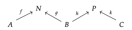
Then, if a pushout of \(N \stackrel{g}{\rightarrow} B \stackrel{h}{\leftarrow} P\) exists in C, as shown on the left, we can extract a new cospan in C, as shown on the right:

It might look like we have achieved our goal, but we’re missing some things. First, we need an identity on every object C \(\in\) Ob C; but that’s not hard: use C → C ← C where both maps are identities in C. More importantly, we don’t know that C has all pushouts, so we don’t know that every two sequential morphisms A → B → C can be composed. And beyond that, there is a technical condition that when we form pushouts, we only get an answer ‘up to isomorphism’: anything isomorphic to a pushout counts as a pushout (check the definition to see why). We want all these different choices to count as the same thing, so we define two cospans to be equivalent iff there is an isomorphism between their respective apexes. That is, the cospan A → P ← B and A → P′ ← B in the diagram shown left below are equivalent iff there is an isomorphism P \(\cong\) P′ making the diagram to the right commute:

Now we are getting somewhere. As long as our category C has pushouts, we are in business: Cospan\(_{C}\) will form a category. But in fact, we are very close to getting more. If we also demand that C has an initial object Ø as well, then we can upgrade Cospan\(_{C}\) to a symmetric monoidal category.

Recall from Proposition 6.32 that a category C has all finite colimits iff it has an initial object and all pushouts.

Definition 6.45.

Let C be a category with finite colimits. Then there exists a category Cospan\(_{C}\) with the same objects as C, i.e. Ob(Cospan\(_{C}\)) = Ob(C), where the morphisms A → B are the (equivalence classes of) cospans from A to B, and composition is given by the above pushout construction.

There is a symmetric monoidal structure on this category, denoted (Cospan\(_{C}\), Ø, +). The monoidal unit is the initial object Ø \(\in\) C and the monoidal product is given by coproduct. The coherence isomorphisms, e.g. A + Ø \(\cong\) A, can be defined in a similar way to those in Exercise 6.18.

It is a straightforward but time-consuming exercise to verify that (Cospan\(_{C}\), Ø, +) from Definition 6.45 really does satisfy all the axioms of a symmetric monoidal category, but it does.

Example 6.46.

The category FinSet has finite colimits (see 6.36). So, we can define a symmetric monoidal category Cospan\(_{FinSet}\). What does it look like? It looks a lot like wires connecting ports.

The objects of Cospan\(_{FinSet}\) are finite sets; here let’s draw them as collections of •’s. The morphisms are cospans of functions. Let A and N be five element sets, and B be a \(A \stackrel{f}{\rightarrow} N \stackrel{g}{\leftarrow} B\).

In the depiction on the left, we simply represent the functions f and g by drawing arrowsfromeacha \(\in\) A to f(a) and each b \(\in\) B to g(b). In the depiction on the right, we make this picture resemble wires a bit more, simply drawing a wire where before we had an arrow, and removing the unnecessary center dots. We also draw a dotted line around points that are connected, to emphasize an important perspective, that cospans establish that certain ports are connected, i.e. part of the same equivalence class.

The monoidal category Cospan\(_{FinSet}\) then provides two operations for combining cospans: composition and monoidal product. Composition is given by taking the pushout of the maps coming from the common foot, as described in Definition 6.45. Here is an example of cospan composition, where all the functions are depicted with arrow notation:

The monoidal product is given simply by the disjoint union of two cospans; in pictures it is simply combining two cospans by stacking one above another.

Exercise 6.48.

In Eq. (6.47) we showed morphisms A → B and B → C in Cospan\(_{FinSet}\).

Draw their monoidal product as a morphism A + B → B + C in Cospan\(_{FinSet}\). ♦

Exercise 6.49.

Depicting the composite of cospans in Eq. (6.47) with the wire notation gives

Comparing Eq. (6.47) and Eq. (6.50), describe the composition rule in Cospan\(_{FinSet}\) in terms of wires and connected components. ♦