6.4: Decorated cospans

The goal of this section is to show how we can construct a hypergraph category whose morphisms are electric circuits. To do this, we first must introduce the notion of structure-preserving map for symmetric monoidal categories, a generalization of monoidal monotones known as symmetric monoidal functors. Then we introduce a general method that of decorated cospans for producing hypergraph categories. Doing all this will tie up lots of loose ends: colimits, cospans, circuits, and hypergraph categories.

Symmetric monoidal functors

Rough Definition 6.68.

Let (C, I\(_{C}\), ⊗\(_{C}\)) and (D, I\(_{D}\), ⊗\(_{D}\)) be symmetric monoidal cate- gories. To specify a symmetric monoidal functor (F, φ) between them,

(i) one specifies a functor F : C → D;

(ii) one specifies a morphism φ\(_{I}\) : I\(_{D}\) → F(I\(_{C}\)).

(iii) for each c\(_{1}\), c\(_{2}\) \(\in\) Ob(C), one specifies a morphism

φ\(_{c1,c2}\) : F(c\(_{1}\)) ⊗\(_{D}\) F(c\(_{2}\)) → F(c\(_{1}\) ⊗\(_{C}\) c\(_{2}\)),

natural in c\(_{1}\) and c\(_{2}\).

We call the various maps φ coherence maps.

We require the coherence maps to obey bookkeeping axioms that ensure they are well behaved with respect to the symmetric monoidal structures on C and D. If φ\(_{I}\) and φ\(_{c1,c2}\) are isomorphisms for all c\(_{1}\), c\(_{2}\), we say that (F, φ) is strong.

Example 6.69.

Consider the power set functor P: Set → Set. It acts on objects by sending a set S \(\in\) Set to its set of subsets P(S) := {R \(\subseteq\) S}. It acts on morphisms by sending a function f : S → T to the image map imf : P(S) → P(T), which maps R \(\subseteq\) S to {f (r) | r \(\in\) R} \(\subseteq\) T.

Now consider the symmetric monoidal structure ({1}, ×) on Set from Example 4.49. To make P a symmetric monoidal functor, we need to specify a function φ\(_{I}\) : {1} → P({1}) and for all sets S and T, a functor φ\(_{S,T}\) : P(S) × P(T) → P(S × T). One possibility is to define φ\(_{I}\)(1) to be the maximal subset {1} \(\subseteq\) {1}, and given subsets A \(\subseteq\) S and B \(\subseteq\) T, to define φ\(_{S,T}\)(A, B) to be the product subset A × B \(\subseteq\) S × T. With these definitions, (P, φ) is a symmetric monoidal functor.

Exercise 6.70.

Check that the maps φ\(_{S,T}\) defined in Example 6.69 are natural in S and T. In other words, given f : S → S′ and g: T → T′, show that the diagram below commutes:

♦

Decorated cospans

Now that we have briefly introduced symmetric monoidal functors, we return to the task at hand: constructing a hypergraph category of circuits. To do so, we introduce the method of decorated cospans.

Circuits have lots of internal structure, but they also have some external ports also called ‘terminals’ by which to interconnect them with others. Decorated cospans are ways of discussing exactly that: things with external ports and internal structure.

To see how this works, let us start with the following example circuit:

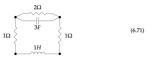
We might formally consider this as a graph on the set of four ports, where each edge is labeled by a type of circuit component (for example, the top edge would be labeled as a resistor of resistance 2Ω). For this circuit to be a morphism in some category, i.e. in order to allow for interconnection, we must equip the circuit with some notion of interface. We do this by marking the ports in the interface using functions from finite sets:

Let N be the set of nodes of the circuit. Here the finite sets A, B, and N are sets consisting of one, two, and four elements respectively, drawn as points, and the values of the functions A → N and B → N are indicated by the grey arrows. This forms a cospan in the category of finite sets, for which the apex set N has been decorated by our given circuit.

Suppose given another such decorated cospan with input B

Since the output of the first equals the input of the second (both are B), we can stick them together into a single diagram:

The composition is given by gluing the circuits along the identifications specified by B, resulting in the decorated cospan

We’ve seen this sort of gluing before when we defined composition of cospans in Definition 6.45. But now there’s this whole ‘decoration’ thing; our goal is to formalize it.

Definition 6.75.

Let C be a category with finite colimits, and (F, φ) : (C, +) → (Set, ×) be a symmetric monoidal functor. An F-decorated cospan is a pair consisting of a cospan \(A \stackrel{i}{\rightarrow} N \stackrel{o}{\leftarrow} B\) in C together with an element s ∈ F(N).5 We call (F, φ) the decoration functor and s the decoration.

The intuition here is to use C = FinSet, and, for each object N \(\in\) FinSet, the functor F assigns the set of all legal decorations on a set N of nodes. When you choose an F decorated cospan, you choose a set A of left-hand external ports, a set B of right-hand external ports, each of which maps to a set N of nodes, and you choose one of the available decorations on N nodes, taken from the set F(N).

So, in our electrical circuit case, the decoration functor F sends a finite set N to the set of circuit diagrams graphs whose edges are labeled by resistors, capacitors, etc.—that have N vertices. Our goal is still to be able to compose such diagrams; so how does that work exactly?

Basically one combines the way cospans are composed with the structures defining our decoration functor: namely F and φ.

Let (\(A \stackrel{f}{\rightarrow} N \stackrel{g}{\leftarrow} B\),s) and (\(B \stackrel{h}{\rightarrow} P \stackrel{k}{\leftarrow} C\), t) represent decorated cospans. Their composite is represented by the composite of the cospan \(A \stackrel{f}{\rightarrow} N \stackrel{g}{\leftarrow} B\) and \(B \stackrel{h}{\rightarrow} P \stackrel{k}{\leftarrow} C\), paired with the following element of F(N +\(_{B}\) P):

\(F\left(\left[\iota_{N}, \iota_{P}\right]\right)\left(\varphi_{N, P}(s, t)\right)\) (6.76)

That’s rather compact! We’ll unpack it, in a concrete case, in just a second. But let’s record a theorem first.

Theorem 6.77.

Given a category C with finite colimits and asymmetric monoidal functor (F, φ) : (C, +) → (Set, ×), there is a hypergraph category Cospan\(_{F}\) whose objects are the objects of C, and whose morphisms are equivalence classes of F-decorated cospans.

The symmetric monoidal and hypergraph structures are derived from those on Cospan\(_{C}\).

Exercise 6.78.

Suppose you’re worried that the notation Cospan\(_{C}\) looks like the notation Cospan\(_{F}\), even though they’re very different. An expert tells you “they’re not so different; one is a special case of the other. Just use the constant functor F(c) := {∗}.” What does the expert mean?

Electric circuits

In order to work with the above abstractions, we will get a bit more precise about the circuits example and then have a detailed look at how composition works in decorated cospan categories.

Let’s build some circuits. To begin, we’ll need to choose which components we want in our circuit. This is simply a matter of what’s in our electrical toolbox. Let’s say we’re carrying some lightbulbs, switches, batteries, and resistors of every possible resistance. That is, define a set

\(C:=\{\text { light, switch, battery }\} \sqcup\left\{x \Omega \mid x \in \mathbb{R}^{+}\right\}\)

To be clear, the Ω are just labels; the above set is isomorphic to {light, switch, battery}⊔ \(\mathbb{R}\)+. But we write C this way to remind us that it consists of circuit components. If we wanted, we could also add inductors, capacitors, and even elements connecting more than two ports, like transistors, but let’s keep things simple for now.

Given our set C, a C-circuit is just a graph (V, A, s, t), where s,t : A → V are the source and target functions, together with a function l : A → C labeling each edge with a certain circuit component from C.

For example, we might have the simple case of V = {1,2}, A = {e}, s(e) = 1, t(e) = 2 so e is an edge from 1 to 2 and l(e) = 3Ω. This represents a resistor with resistance 3Ω:

Note that in the formalism we have chosen, we have multiple ways to represent any circuit, as our representations explicitly choose directions for the edges. The above resistor could also be represented by the ‘reversed graph’, with data V = {1, 2}, A = {e}, s(e) = 2, t(e) = 1, and l(e) = 3F.

Exercise 6.79.

Write a tuple (V, A, s, t, l) that represents the circuit in Eq. (6.71). ♦

A decoration functor for circuits. We want C-circuits to be our decorations, so let’s use them to define a decoration functor as in Definition 6.75.

We’ll call the functor (Circ, ψ). We start by defining the functor part

Circ : (FinSet, +) → (Set, ×)

as follows. On objects, simply send a finite set V to the set of C-circuits:

Circ(V) := {(V, A, s, t, l) | where s,t : A → V, l : E → C}.

On morphisms, Circ sends a function f : V → V′ to the function

Circ( f ) : Circ(V) → Circ(V′);

(V, A, s, t, l) \(\longmapsto\) (V', A, (s ; f), (t ; f), l).

This defines a functor; let’s explore it a bit in an exercise.

Exercise 6.80.

To understand this functor better, let c \(\in\) Circ(\(\underline{4}\)) be the circuit

and let f :\(\underline{4}\) → \(\underline{3}\) be the function

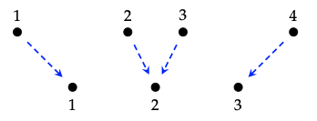
Draw a picture of the circuit Circ( f )(c). ♦

We’re trying to get a decoration functor (Circ, ψ) and so far we have Circ. For the coherence maps ψ\(_{V,V'}\) for finite sets V, V′, we define

\(\begin{array}{c}
\psi_{V, V^{\prime}}: \operatorname{Circ}(V) \times \operatorname{Circ}\left(V^{\prime}\right) \longrightarrow \operatorname{Circ}\left(V+V^{\prime}\right) \\
\left((V, A, s, t, \ell),\left(V^{\prime}, A^{\prime}, s^{\prime}, t^{\prime}, \ell^{\prime}\right)\right) \longmapsto\left(V+V^{\prime}, A+A^{\prime}, s+s^{\prime}, t+t^{\prime},\left[\ell, \ell^{\prime}\right]\right)
\end{array}\) (6.81)

This is simpler than it may look: it takes a circuit on V and a circuit on V′, and just considers them together as a circuit on the disjoint union of vertices V + V′.

Exercise 6.82.

Suppose we have circuits

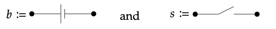
in Circ(\(\underline{2}\)).

Use the definition of ψ\(_{V,V'}\) from (6.81) to figure out what 4-vertex circuit ψ\(_{\underline{2},\underline{2}}\)(b, s) \(\in\) Circ(\(\underline{2}\) + \(\underline{2}\)) = Circ(\(\underline{4}\)) should be, and draw a picture. ♦

Open circuits using decorated cospans. From the above data, just a monoidal functor (Circ, ψ) : (FinSet, +) → (Set, ×), we can construct our promised hypergraph category of circuits!

Our notation for this category is Cospan\(_{Circ}\). Following Theorem 6.77, the objects of this category are the same as the objects of FinSet, just finite sets. We’ll reprise our notation from the introduction and Example 6.42, and draw these finite sets as collections of white circles ◦.

For example, we’ll represent the object 2 of Cospan\(_{Circ}\) as two white circles:

These white circles mark interface points of an open circuit.
More interesting than the objects, however, are the morphisms in Cospan\(_{Circ}\).

These are open circuits. By Theorem 6.77, a morphism \(\underline{m}\) → \(\underline{n}\) is a Circ-decorated cospan: that is, cospan \(\underline{m}\) → \(\underline{p}\) ← \(\underline{n}\) together with an element c of Circ(\(\underline{p}\)).

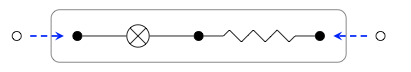
As an example, consider the cospan \(\underline{1} \stackrel{i_{1}}{\rightarrow} \underline{2} \stackrel{i_{2}}{\leftarrow} \underline{1}\) where i\(_{1}\)(1) = 1 and i\(_{2}\)(1) = 2, equipped with the battery element of Circ(\(\underline{2}\)) connecting node 1 and node 2. We’ll depict this as follows:

Exercise 6.84.

Morphisms of Cospan\(_{Circ}\) are Circ-decorated cospans, as defined in Definition 6.75. This means (6.83) depicts a cospan together with a decoration, which is some C-circuit (V, A, s, t, l) \(\in\) Circ(\(\underline{2}\)). What is it? ♦

Let’s now see how the hypergraph operations in Cospan\(_{Circ}\) can be used to construct electric circuits.

Composition in Cospan\(_{Circ}\). First we’ll consider composition. Consider the following decorated cospan from \(\underline{1}\) to \(\underline{1}\):

Since this and the circuit in (6.83) are both morphisms \(\underline{1}\) → \(\underline{1}\), we may compose them to get another morphism \(\underline{1}\) → \(\underline{1}\). How do we do this? There are two parts: to get the new cospan, we simply compose the cospans of our two circuits, and to get the new decoration, we use the formula Circ([ι\(_{N}\) , ι\(_{P}\)])(ψ\(_{N,P}\)(s, t)) from (6.76). Again, this is rather compact! Let’s unpack it together.

We’ll start with the cospans. The cospans we wish to compose are

We simply ignore the decorations for now.) If we pushout over the common set 1 = {◦}, we obtain the pushout square

This means the composite cospan is

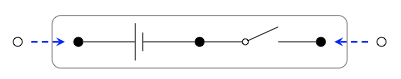
In the meantime, we already had you start us off unpacking the formula for the new decoration. You told us what the map ψ\(_{\underline{2},\underline{2}}\) does in Exercise 6.82. It takes the two decorations, both circuits in Circ(\(\underline{2}\)), and turns them into the single, disjoint circuit

in Circ(\(\underline{4}\)). So this is what the ψ\(_{N,P}\)(s, t) part means. What does the [ι\(_{N}\) , ι\(_{P}\)] mean? Recall this is the copairing of the pushout maps, as described in Examples 6.14 and 6.25. In our case, the relevant pushout square is given by (6.85), and [ι\(_{N}\) , ι\(_{P}\)] is in fact the function f from Exercise 6.80!

This means the decoration on the composite cospan is

Putting this all together, the composite circuit is

Exercise 6.86.

Refer back to the example at the beginning of Section 6.4.2. In particular, consider the composition of circuits in Eq. (6.73). Express the two circuits in this diagram as morphisms in Cospan\(_{Circ}\), and compute their composite. Does it match the picture in Eq. (6.74)? ♦

Monoidal products in Cospan\(_{Circ}\). Monoidal products in Cospan\(_{Circ}\) are much sim- pler than composition. On objects, we again just work as in FinSet: we take the disjoint union of finite sets. Morphisms again have a cospan, and a decoration.

For cospans, we again just work in Cospan\(_{FinSet}\): given two cospans A → M ← B and C → N ← D, we take their coproduct cospan A + C → M + N ← B + D. And for decorations, we use the map ψ\(_{M,N}\) : Circ(M) × Circ(N) → Circ(M + N). So, for example, suppose we want to take the monoidal product of the open circuits

and

The result is given by stacking them. In other words, their monoidal product is:

Easy, right?

We leave you to do two compositions of your own.

Exercise 6.88.

Write x for the open circuit in (6.87). Also define cospans η : 0 → 2 and η : 2 → 0 as follows:

where each of these are decorated by the empty circuit (1, Ø, !, !, !) \(\in\) Circ(\(\underline{1}\)).\(^{6}\)

Compute the composite η ; x ; ε in Cospan\(_{Circ}\). This is a morphism \(\underline{0}\) → \(\underline{0}\); we call such things closed circuits. ♦