6.5: Operads and their algebras

In Theorem 6.77 we described how decorating cospans builds a hypergraph category from a symmetric monoidal functor. We then explored how that works in the case that the decoration functor is somehow “all circuit graphs on a set of nodes”.

In this book, we have devoted a great deal of attention to different sorts of composi- tional theories, from monoidal preorders to compact closed categories to hypergraph categories. Yet for an application you someday have in mind, it may be the case that none of these theories suffice. You need a different structure, customized to a particular situation. For example in [VSL15] the authors wanted to compose continuous dynam- ical systems with control-theoretic properties and realized that in order for feedback to make sense, the wiring diagrams could not involve what they called ‘passing wires’.

So to close our discussion of compositional structures, we want to quickly sketch something we can use as a sort of meta-compositional structure, known as an operad. We saw in Section 6.4.3 that we can build electric circuits from a symmetric monoidal functor FinSet → Set. Similarly we’ll see that we can build examples of new algebraic structures from operad functors O → Set.

Operads design wiring diagrams

Understanding that circuits are morphisms in a hypergraph category is useful: it means we can bring the machinery of category theory to bear on understanding electrical circuits. For example, we can build functors that express the compositionality of circuit semantics, i.e. how to derive the functionality of the whole from the functionality and interaction pattern of the parts. Or we can use the category-theoretic foundation to relate circuits to other sorts of network systems, such as signal flow graphs. Finally, the basic coherence theorems for monoidal categories and compact closed categories tell us that wiring diagrams give sound and complete reasoning in these settings.

However, one perhaps unsatisfying result is that the hypergraph category intro- duces artifacts like the domain and codomain of a circuit, which are not inherent to the structure of circuits or their composition. Circuits just have a single boundary interface, not ‘domains’ and ‘codomains’. This is not to say the above model is not useful: in many applications, a vector space does not have a preferred basis, but it is often useful to pick one so that we may use matrices (or signal flow graphs!). But it would be worthwhile to have a category-theoretic model that more directly represents the compositional structure of circuits. In general, we want the category-theoretic model to fit our desired application like a glove. Let us quickly sketch how this can be done.

Let’s return to wiring diagrams for a second. We saw that wiring diagrams for hypergraph categories basically look like this:

Note that if you had a box with A and B on the left and D on the right, you could plug the above diagram right inside it, and get a new open circuit. This is the basic move of operads.

But before we explain this, let’s get where we said we wanted to go: to a model where there aren’t ports on the left and ports on the right, there are just ports. We want a more succinct model of composition for circuit diagrams; something that looks more like this:

Do you see how diagrams Eq. (6.89) and Eq. (6.90) are actually exactly the same in

terms of interconnection pattern? The only difference is that the latter does not have left/right distinction: we have lost exactly what we wanted to lose.

The cost is that the ‘boxes’ f , g, h, k in Eq. (6.90) no longer have a left/right dis- tinction; they’re just circles now. That wouldn’t be bad except that it means they can no longer represent morphisms in a category—like they used to above, in Eq. (6.89) because morphisms in a category by definition have a domain and codomain. Our new circles have no such distinction. So now we need a whole new way to think about ‘boxes’ categorically: if they’re no longer morphisms in a category, what are they? The answer is found in the theory of operads.

In understanding operads, we will find we need to navigate one of the level shifts that we first discussed in Section 1.4.5. Notice that for decorated cospans, we define a hypergraph category using a symmetric monoidal functor. This is reminiscent of our brief discussion of algebraic theories in Section 5.4.2, where we defined something called the theory of monoids as a prop M, and define monoids using functors M → Set; see Remark 5.74.

In the same way, we can view the category Cospan\(_{FinSet}\) as some sort of ‘theory of hypergraph categories’, and so define hypergraph categories as functors Cospan\(_{FinSet}\) → Set.

So that’s the idea. An operad O will define a theory or grammar of composition, and operad functors O → Set, known as O-algebras, will describe particular applications that obey that grammar.

Rough Definition 6.91.

To specify an operad O,

(i) one specifies a collection T, whose elements are called types;

(ii) for each tuple (t\(_{1}\), ..., t\(_{n}\),t) of types, one specifies a set O(t\(_{1}\), ..., t\(_{n}\) ;t), whose elements are called operations of arity (t\(_{1}\), . . . , t\(_{n}\) ; t);

(iii) for each pair of tuples (s\(_{1}\), ..., s\(_{m}\), t\(_{i}\)) and (t\(_{1}\), ..., t\(_{n}\), t), one specifies a function

◦ \(_{i}\) : O(s\(_{1}\), ..., s\(_{m}\); t\(_{i}\)) × O(t\(_{1}\), ..., t\(_{n}\); t) → O(t\(_{1}\), ..., t\(_{i-1}\), s\(_{1}\), ..., s\(_{m}\), t\(_{i+1}\), ..., t\(_{n}\) ; t);

called substitution; and

(iv) for each type t, one specifies an operation id\(_{t}\) \(\in\) O(t ; t) called the identity operation.

These must obey generalized identity and associativity laws.

Let’s ignore types for a moment and think about what this structure models. The intuition is that an operad consists of, for each n, a set of operations of arity n that is, all the operations that accept n arguments. If we take an operation f of arity m, and plug the output into the i th argument of an operation g of arity n, we should get an operation of arity m + n − 1: we have m arguments to fill in m, and the remaining n − 1 arguments to fill in m. Which operation of aritym + n − 1 do we get? This is described by the substitution function ◦\(_{i}\), which says we obtain the operation f ◦\(_{i}\)g \(\in\) O(m + n − 1). The coherence conditions say that these functions ◦\(_{i}\) capture the following intuitive picture:

The types then allow us to specify the, well, types of the arguments inputs that each function takes. So making tea is a 2-ary operation, an operation with arity 2, because it takes in two things. To make tea you need some warm water, and you need some tea leaves.

Example 6.92.

Context-free grammars are to operads as graphs are to categories. Let’s sketch what this means. First, a context-free grammar is a way of describing a particular set of ‘syntactic categories’ that can be formed from a set of symbols. For example, in English we have syntactic categories like nouns, determiners, adjectives, verbs, noun phrases, prepositional phrases, sentences, etc. The symbols are words, e.g. cat, dog, the, chases.

To define a context-free grammar on some alphabet, one specifies some production rules, which say how to form an entity in some syntactic category from a bunch of entities in other syntactic categories. For example, we can form a noun phrase from a determiner (the), an adjective (happy), and a noun (boy). Context free grammars are important in both linguistics and computer science. In the former, they’re a basic way to talk about the structure of sentences in natural languages. In the latter, they’re crucial when designing parsers for programming languages.

So just like graphs present free categories, context-free grammars present free operads. This idea was first noticed in [HMP98].

Operads from symmetric monoidal categories

We will see in Definition 6.97 that a large class of operads come from symmetric monoidal categories. Before we explain this, we give a couple of examples. Perhaps the most important operad is that of Set.

Example 6.93.

The operad Set of sets has

(i) Sets X as types.

(ii) Functions X\(_{1}\) × ··· × X\(_{n}\) →Y as operations of arity (X\(_{1}\), ..., X\(_{n}\) ; Y).

(iii) Substitution defined by

(g ◦ \(_{i}\)f )(x\(_{1}\), ..., x\(_{i-1}\), w\(_{1}\), ..., w\(_{m}\), x\(_{i+1}\), ..., x\(_{n}\))
= g (x\(_{1}\), ..., x\(_{i-1}\), f (w\(_{1}\), ..., w\(_{m}\)), x\(_{i+1}\), ..., x\(_{n}\)

where f \(\in\) Set(W\(_{1}\), ..., W\(_{m}\); X\(_{i}\)), g \(\in\) Set(X\(_{1}\), ..., X\(_{n}\) ; Y), and hence g ◦\(_{i}\) f is a function

(g ◦\(_{i}\) f ): X\(_{1}\) × ··· × X\(_{i-1}\) ×W\(_{1}\) × ··· × W\(_{m}\) × X\(_{i+1}\) × ··· × X\(_{n}\) →Y

(iv) Identities id\(_{X}\) \(\in\) Set(X ; X) are given by the identity function id\(_{X}\) : X → X.

Next we give an example that reminds us what all this operad stuff was for: wiring diagrams.

Example 6.94.

The operad Cospan of finite-set cospans has

(i) Natural numbers a \(\in\) \(\mathbb{N}\) as types.

(ii) Cospans a\(\underline{_{1}}\) + ··· + a\(\underline{_{n}}\) → p ← b of finite sets as operations of arity (a\(_{1}\), ..., a\(_{n}\) ; b).

(iii) Substitution defined by pushout.

(iv) Identities id\(_{a}\) \(\in\) Set(a; a) just given by the identity cospan \(\underline{a}\) \stackrel{id\(_{\underline{a}}\){\rightarrow} \(\underline{a}\) \stackrel{id\(_{\underline{a}}\)}{\leftarrow} \(\underline{a}\)\).

This is the operadic analogue of the monoidal category (Cospan\(_{FinSet}\) , 0, +).

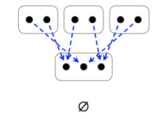
We can depict operations in this operad using diagrams like we drew above. For example, here’s a picture of an operation:

This is an operation of arity (\(\underline{3}\), \(\underline{3}\), \(\underline{4}\), \(\underline{2}\); 3). Why? The circles marked f and g have 3 ports, h has 4 ports, k has 2 ports, and the outer circle has 3 ports: 3, 3, 4, 2; 3.

So how exactly is Eq. (6.95) a morphism in this operad?

Well a morphism of this \(\underline{3}\) + \(\underline{3}\) + \(\underline{4}\) + \(\underline{2}\) \stackrel{a}{\rightarrow} \underline{p} \stackrel{b}{\leftarrow} \underline{3}\).

In the diagram above, the apex \(\underline{p}\) is the set \(\underline{7}\), because there are 7 nodes • in the diagram. The function a sends each port on one of the small circles to the node it connects to, and the function b sends each port of the outer circle to the node it connects to.

We are able to depict each operation in the operad Cospan as a wiring diagram. It is often helpful to think of operads as describing a wiring diagram grammar. The substitution operation of the operad signifies inserting one wiring diagram into a circle or box in another wiring diagram.

Exercise 6.96.

1. Consider the following cospan f \(\in\) Cospan(2, 2; 2):

Draw it as a wiring diagram with two inner circles, each with two ports, and one outer circle with two ports.

2. Draw the wiring diagram corresponding to the following cospan g \(\in\) Cospan(2, 2, 2; 0):

3. Compute the cospan g ◦\(_{1}\) f . What is its arity?

4. Draw the cospan g ◦\(_{1}\) f . Do you see it as substitution? ♦

We can turn any symmetric monoidal category into an operad in a way that gener- alizes the above two examples.

Definition 6.97.

For any symmetric monoidal category (C, I, ⊗), there is an operad O\(_{C}\), called the operad underlying C, defined as having:

(i) Ob(C) as types.

(ii) morphisms C\(_{1}\) ⊗ ··· ⊗ C\(_{n}\) →D in C as the operations of arity (C\(_{1}\), ..., C\(_{n}\) ; D).

(iii) substitution is defined by

(f ◦\(_{i}\) g) := f ◦ (id, ..., id, g, id, ..., id)

(iv) identities id\(_{a}\) \(\in\) O\(_{C}\)(a ; a) defined by id\(_{a}\).

We can also turn any monoidal functor into what’s called an operad functor.

The operad for hypergraph props

An operad functor takes the types of one operad to the types of another, and then the op- erations of the first to the operations of the second in a way that respects this.

Rpugh Definition 6.98.

Suppose given two operads O and P with type collections T and U respectively. To specify an operad functor F : O → P,

(i) one specifies a function f : T → U.
(ii) For all arities (t\(_{1}\), . . . , t\(_{n}\) ; t) in O, one specifies a function

F : O(t\(_{1}\), ..., t\(_{n}\) ; t) → P(f (t\(_{1}\)), ..., f (t\(_{n}\)) ; f (t))

such that composition and identities are preserved.

Just as set-valued functors C → Set from any category C are of particular interest— we saw them as database instances in Chapter 3 so to are Set-valued functors O → Set from any operad O.

Definition 6.99.

An algebra for an operad O is an operad functor F : O → Set.

We can think of functors O → Set as defining a set of possible ways to fill the boxes in a wiring diagram. Indeed, each box in a wiring diagram represents a type t of the given operad O and an algebra F : O → Set will take a type t and return a set F(t) of fillers for box t. Moreover, given an operation (i.e., a wiring diagram) f \(\in\) O(t1, . . . , tn; t), we get a function F(f) that takes an element of each set F(ti), and returns an element of F(t). For example, it takes n circuits with interface t1, . . . , tn respectively, and returns a circuit with boundary t.

Example 6.100.

For electric circuits, the types are again finite sets, T = Ob(FinSet), where each finite set t \(\in\) T corresponds to a cell with t ports. Just as before, we have a set Circ(t) of fillers, namely the set of electric circuits with that t-marked terminals. As an operad algebra, Circ : Cospan → Set transforms wiring diagrams like this one

into formulas that build a new circuit from a bunch of existing ones.

In the above drawn case, we would get a morphism Circ(φ) \(\in\) Set(Circ(2), Circ(2), Circ(2); Circ(0)), i.e. a function

Circ(φ) : Circ(2) × Circ(2) × Circ(2) → Circ(0).

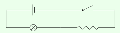
We could apply this function to the three elements of Circ(2) shown here

and the result would be the closed circuit from the beginning of the chapter:

This is reminiscent of the story for decorated cospans: gluing fillers together to form hypergraph categories. An advantage of the decorated cospan construction is that one obtains an explicit category (where morphisms have domains and codomains and can hence be composed associatively), equipped with Frobenius structures that allow us to get around the strictures of domains and codomains. The operad perspective has other advantages. First, whereas decorated cospans can produce only some hypergraph categories, Cospan-algebras can produce any hypergraph category.

Proposition 6.101.

There is an equivalence between Cospan-algebras and hypergraph props.

Another advantage of using operads is that one can vary the operad itself, from Cospan to something similar (like the operad of ‘cobordisms’), and get slightly different compositionality rules.

In fact, operads with the additional complexity in their definition—can be cus- tomized even more than all compositional structures defined so far. For example, we can define operads of wiring diagrams where the wiring diagrams must obey precise conditions far more specific than the constraints of a category, such as requiring that the diagram itself has no wires that pass straight through it. In fact, operads are strong enough to define themselves: roughly speaking, there is an operad for operads: the category of operads is equivalent to the category of algebras for a certain operad [Lei04, Example 2.2.23]. While operads can, of course, be generalized again, they conclude our march through an informal hierarchy of compositional structures, from preorders to categories to monoidal categories to operads.