6.3: Hyper Graph Categories

A hypergraph category is a type of symmetric monoidal category whose wiring diagrams are networks. We will soon see that electric circuits can be organized into a hypergraph category; this is what we’ve been building up to. But to define hypergraph categories, it is useful to first introduce Frobenius monoids.

Frobenius monoids

The pictures of cospans we saw above, e.g. in Eq. (6.50) look something like icons in signal flow graphs (see Section 5.3.2): various wires merge and split, initialize and terminate. And these follow the same rules they did for linear relations, which we briefly discussed in Exercise 5.84. There’s a lot of potential for confusion, so let’s start from scratch and build back up.

In any symmetric monoidal category (C, I, ⊗), recall from Section 4.4.2 that objects can be drawn as wires and morphisms can be drawn as boxes. Particularly noteworthy morphisms might be iconified as dots rather than boxes, to indicate that the morphisms there are not arbitrary but notation-worthy. One case of this is when there is an object X with special “abilities”, e.g. the ability to duplicate into two, or disappear into nothing. To make this precise, recall from Definition 5.65 that a commutative monoid (X, μ, η) in symmetric monoidal category (C, I, ⊗) is an object X of C together with (noteworthy) morphisms

obeying

where is the symmetry on X ⊗ X. A cocommutative cocomonoid (X, δ, ε) is an object X with maps δ : X → X ⊗ X, ε : X → I, obeying the mirror images of the laws in Eq. (6.51).

Suppose X has both the structure of a commutative monoid and cocommutative comonoid, and consider a wiring diagram built only from the icons μ, η, δ, and ε, where every wire is labeled X. These diagrams have a left and right, and are pictures of how ports on the left are connected to ports on the right. The commutative monoid and cocommutative comonoid axioms thus both express when to consider two such connection pictures should be considered the same. For example, associativity says the order of connecting ports on the left doesn’t matter; coassociativity (not drawn) says the same for the right.

If you want to go all the way and say “all I care about is which port is connected to which; I don’t even care about left and right”, then you need a few more axioms to say how the morphisms μ and δ, the merger and the splitter, interact.

Definition 6.52.

Let X be an object in a symmetric monoidal category (C, ⊗, I). A Frobe- nius structure on X consists of a 4-tuple (μ, η, δ, ε) such that (X, μ, η) is a commutative monoid and (X, δ, ε) is a cocommutative comonoid, which satisfies the six equations above ((co-)associativity, (co-)unitality, (co-)commutativity), as well as the following three equations:

We refer to an object X equipped with a Frobenius structure as a special commutative Frobenius monoid, or just Frobenius monoid for short.

With these two equations, it turns out that two morphisms X ⊗ m → X ⊗ n defined by composing and tensoring identities on X and the noteworthy morphisms μ, δ, etc.— are equal if and only if their string diagrams connect the same ports. This link between connectivity, and Frobenius monoids can be made precise as follows.

Definition 6.54.

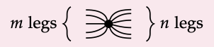
Let (X, μ, η, δ, ε) be a Frobenius monoid in a monoidal category (C, I, ⊗). Let m, n ∈ N. Define sm,n : X⊗m → X⊗n to be the following morphism

It can be written formally as (m − 1) μ’s followed by (n − 1) δ’s, with special cases when m = 0 or n = 0.

We call s\(_{m,n}\) the spider of type (m, n), and can draw it more simply as the icon

So a special commutative Frobenius monoid, aside from being a mouthful, is a ‘spiderable’ wire. You agree that in any monoidal category wiring diagram language, wires represent objects and boxes represent morphisms? Well in our weird way of talking, if a wire is spiderable, it means that we have a bunch of morphisms μ, η, δ, ε, σ that we can combine without worrying about the order of doing so: the result is just “how many in’s, and how many out’s”: a spider. Here’s a formal statement.

Theorem 6.55.

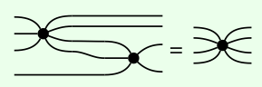
Let (X, μ, η, δ, ε) be a Frobenius monoid in a monoidal category (C, I, ⊗). Suppose that we have a map f : X ⊗ m → X ⊗ n each constructed from spiders and the symmetry map σ: X ⊗ 2 → X ⊗ 2 using composition and the monoidal product, and such that the string diagram of f has only one connected component. Then it is a spider: f = s\(_{m,n}\).

Example 6.56.

As the following two morphisms both (i) have the same number of inputs and outputs, (ii) are constructed only from spiders, and (iii) are connected, Theorem 6.55 immediately implies they are equal:

Example 6.57.

Let X be an object equipped with a Frobenius structure. Which of the morphisms X ⊗ X → X ⊗ X ⊗ X in the following list are necessarily equal?

♦

Back to cospans. Another way of understanding Frobenius monoids is to relate them to cospans. Recall the notion of prop presentation from Definition 5.33.

Theorem 6.58.

Consider the four-element set G := {μ, η, δ, ε} and define in, out : G → N as follows:

\(\begin{array}{cccc}
\operatorname{in}(\mu):=2, & \operatorname{in}(\eta):=0, & \operatorname{in}(\delta):=1, & \operatorname{in}(\epsilon):=1, \\
\operatorname{out}(\mu):=1, & \operatorname{out}(\eta):=1, & \text { out }(\delta):=2, & \operatorname{out}(\epsilon):=0 .
\end{array}\)

Let E be the set of Frobenius axioms, i.e. the nine equations from Definition 6.52.

Then the free prop on (G,E) is equivalent, as a symmetric monoidal category,a to Cospan\(_{FinSet}\).

Thus we see that ideal wires, connectivity, cospans, and objects with Frobenius structures are all intimately related. We use Frobenius structures (all that splitting, merging, initializing, and terminating stuff) as a way to capture the grammar of circuit diagrams.

Wiring diagrams for hypergraph categories

We introduce hypergraph categories through their wiring diagrams. Just like for monoidal categories, the formal definition is just the structure required to unambigu- ously interpret these diagrams.

Indeed, our interest in hypergraph categories is best seen in their wiring diagrams. The key idea is that wiring diagrams for hypergraph categories are network diagrams. This means, in addition to drawing labeled boxes with inputs and outputs, as we can for monoidal categories, and in addition to bending these wires around as we can for compact closed categories, we are allowed to split, join, terminate, and initialize wires.

Here is an example of a wiring diagram that represents a composite of morphisms in a hypergraph category

We have suppressed some of the object/wire labels for readability, since all types can be inferred from the labeled ones.

Exercise 6.59.

1. What label should be on the input to h?

2. What label should be on the output of g?

3. What label should be on the fourth output wire of the composite? ♦

Thus hypergraph categories are general enough to talk about all network-style diagrammatic languages, like circuit diagrams.

Definition of hypergraph category

We are now ready to define hypergraph categories formally. Since the wiring diagrams for hypergraph categories are just those for symmetric monoidal categories with a few additional icons, the definition is relatively straightforward: we just want a Frobenius structure on every object. The only coherence condition is that these interact nicely with the monoidal product.

Definition 6.60.

A hypergraph category is a symmetric monoidal category (C, I, ⊗) in which each object X is equipped with a Frobenius structure (X, μ\(_{X}\) , δ\(_{X}\) , η\(_{X}\) , ε\(_{X}\)) such that

for all objects X, Y, and such that η\(_{I}\) = id\(_{I}\) = ε\(_{I}\).
A hypergraph prop is a hypergraph category that is also a prop, e.g. Ob(C) = \(\mathbb{N}\), etc.

Exercise 6.62.

By Example 6.61, the category Cospan\(_{FinSet}\) is a hypergraph category. (In fact, it is equivalent to a hypergraph prop.) Draw the Frobenius morphisms for the object 1 in Cospan\(_{FinSet}\) using both the function and wiring depictions as in Example 6.46. ♦

Exercise 6.63.

Using your knowledge of colimits, show that the maps defined in Example 6.61 do indeed obey the special law (see Definition 6.52). ♦

Example 6.64.

Recall the monoidal category (Corel, Ø, ⊔) from Example 4.61; its objects are finite sets and its morphisms are corelations.

Given a finite set X, define the corelation μ\(_{X}\) : X ⊔ X → X such that two elements of X ⊔ X ⊔ X are equivalent if and only if they come from the same underlying element of X. Define δ\(_{X}\) : X → X ⊔ X in the same way, and define η\(_{X}\) : Ø → X and ε\(_{X}\) : X → Ø such that no two elements of X = Ø ⊔ X = X ⊔ Ø are equivalent.

These maps define a special commutative Frobenius monoid (X, μ\(_{X}\) , δ\(_{X}\) , η\(_{X}\) , ε\(_{X}\)), and in fact give Corel the structure of a hypergraph category.

Example 6.65.

The prop of linear relations, which we briefly mentioned in Exercise 5.84, is a hypergraph category. In fact, it is a hypergraph category in two ways, by choosing either the black ‘copy’ and ‘discard’ generators or the white ‘add’ and ‘zero’ generators as the Frobenius maps.

We can generalize the construction we gave in Theorem 5.87.

Proposition 6.66.

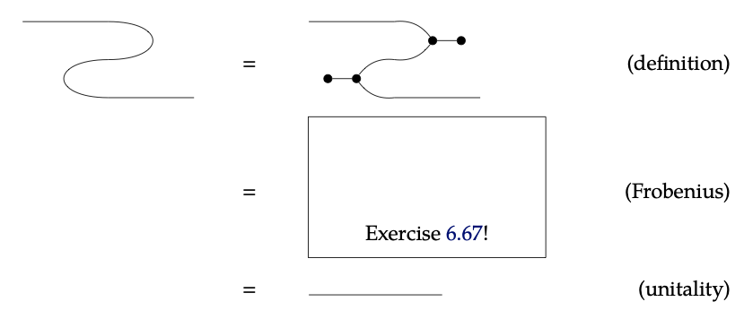
Hypergraph categories are self-dual compact closed categories, if we define the cup and cap to be

Proof. The proof is a straight forward application of the Frobenius and unitality axioms:

\(\square\)

Exercise 6.67.

Fill in the missing diagram in the proof of Proposition 6.66 using the equations from Eq. (6.51), their opposites, and Eq. (6.53). ♦