
3.5: Predicting the Period of a Pendulum
- Page ID
- 58761

Lumping not only turns integration into multiplication, it turns nonlinear into linear differential equations. Our example is the analysis of the period of a pendulum, for centuries the basis of Western timekeeping.
How does the period of a pendulum depend on its amplitude?
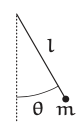
The amplitude \(θ_{0}\) is the maximum angle of the swing; for a loss-less pendulum released from rest, it is also the angle of release. The effect of amplitude is contained in the solution to the pendulum differential equation (see [24] for the equation’s derivation):
\[\frac{d^{2}θ}{dt^{2}} + \frac{g}{l}\sin θ = 0. \label{3.22} \]
The analysis will use all our tools: dimensions (Section 3.5.2), easy cases (Section 3.5.1 and Section 3.5.3), and lumping (Section 3.5.4).
Explain why angles are dimensionless.
Does the pendulum equation have correct dimensions? Use dimensional analysis to show that the equation cannot contain the mass of the bob (except as a common factor that divides out).
Small amplitudes: Applying extreme cases
The pendulum equation is difficult because of its nonlinear factor \(\sin θ\). Fortunately, the factor is easy in the small-amplitude extreme case \(θ \rightarrow 0\). In that limit, the height of the triangle, which is \(\sin θ\), is almost exactly the arclength \(θ\). Therefore, for small angles, \(\sin θ ≈ θ\).
The \(\sin θ ≈ θ\) approximation replaces the arc with a straight, vertical line. To make a more accurate approximation, replace the arc with the chord (a straight but nonvertical line). What is the resulting approximation for \(\sin θ\)?
In the small-amplitude extreme, the pendulum equation becomes linear:
\[\frac{d^{2}θ}{dt^{2}}+\frac{g}{l}θ = 0. \label{3.33} \]
Compare this equation to the spring–mass equation (Section 3.4)
\[\frac{d^{2}x}{dt^{2}}+\frac{k}{m}x = 0. \label{3.34} \]
The equations correspond with \(x\) analogous to \(θ\) and \(k/m\) analogous to \(g/l\). The frequency of the spring-mass system is \(w = \sqrt{k/m}\), and its period is \(T = 2\pi/ω = 2\pi \sqrt{m/k}\). For the pendulum equation, the corresponding period is
\[T = 2\pi\sqrt{\frac{l}{g}} \text{ (for small amplitudes). }\label{3.35} \]
(This analysis is a preview of the method of analogy, which is the subject of Chapter 6.)
Problem 3.26 Checking dimensions
Does the period \(2\pi \sqrt{l/g}\) have correct dimensions?
Problem 3.27 Checking extreme cases
Does the period \(T = 2\pi \sqrt{l/g}\) make sense in the extreme cases \(g \rightarrow \infty\) and \(g \rightarrow 0\)?
Problem 3.28 Possible coincidence
Is it a coincidence that \(g ≈ \pi^{2} m s^{-2}\)? (For an extensive historical discussion that involves the pendulum, see [1] and more broadly also [4, 27, 42].)
Problem 3.29 Conical pendulum for the constant
The dimensionless factor of \(2\pi\) can be derived using an in-sight from Huygens [15, p. 79]: to analyze the motion of a pendulum moving in a horizontal circle (a conical pendulum). Projecting its two-dimensional motion onto a vertical screen produces one-dimensional pendulum motion, so the period of the two-dimensional motion is the same as the period of one-dimensional pendulum motion! Use that idea along with Newton’s laws of motion to explain the \(2\pi\).
Arbitrary amplitudes: Applying Dimensional Analysis
The preceding results might change if the amplitude \(θ_{0}\) is no longer small.
As \(θ_{0}\) increases, does the period increase, remain constant, or decrease?
Any analysis becomes cleaner if expressed using dimensionless groups (Section 2.4.1).
This problem involves the period \(T\), length \(l\), gravitational strength \(g\), and amplitude \(θ_{0}\). Therefore, \(T\) can belong to the dimensionless group \(T/\sqrt{l/g}\). Because angles are dimensionless, \(θ_{0}\) is itself a dimensionless group. The two groups \(T/\sqrt{l/g}\) and \(θ_{0}\) are independent and fully describe the problem (Problem 3.30). An instructive contrast is the ideal spring–mass system. The period \(T\), spring constant \(k\), and mass \(m\) can form the dimensionless group \(T m/k\); but the amplitude \(x_{0}\), as the only quantity containing a length, cannot be part of any dimensionless group (Problem 3.20) and cannot therefore affect the period of the spring–mass system. In contrast, the pendulum’s amplitude \(θ_{0}\) is already a dimensionless group, so it can affect the period of the system.
Check that period \(T\), length \(l\), gravitational strength \(g\), and amplitude \(θ_{0}\) produce two independent dimensionless groups. In constructing useful groups for analyzing the period, why should \(T\) appear in only one group? And why should \(θ_{0}\) not appear in the same group as \(T\)?
Two dimensionless groups produce the general dimensionless form
\[\text{one group = function of the other group}, \label{3.36} \]
so
\[\frac{T}{\sqrt{l/g}} = \text{ function of }θ_{0}. \label{3.37} \]
Because \(T/\sqrt{l/g} = 2\pi\) when \(θ_{0} = 0\) (the small-amplitude limit), factor out the the \(2\pi\) to simplify the subsequent equations, and define a dimensionless period h as follows:
\[\frac{T}{\sqrt{l/g}} = 2\pi h(θ_{0}). \label{3.38} \]
The function \(h\) contains all information about how amplitude affects the period of a pendulum. Using \(h\), the original question about the period becomes the following: Is \(h\) an increasing, constant, or decreasing function of amplitude? This question is answered in the following section.
Large amplitudes: Extreme cases again
For guessing the general behavior of h as a function of amplitude, useful clues come from evaluating \(h\) at two amplitudes. One easy amplitude is the extreme of zero amplitude, where \(h(0) = 1\). A second easy amplitude is the opposite extreme of large amplitudes.
How does the period behave at large amplitudes? As part of that question, what is a large amplitude?
An interesting large amplitude is \(\pi/2\), which means releasing the pendulum from horizontal. However, at \(\pi/2\) the exact \(h\) is the following awful expression (Problem 3.31):
\[h(\pi/2) = \frac{\sqrt{2}}{\pi} \int_{0}^{pi/2} \frac{dθ}{\sqrt{\cos θ}}\label{3.39} \]
Is this integral less than, equal to, or more than 1? Who knows? The integral is likely to have no closed form and to require numerical evaluation (Problem 3.32).
Problem 3.31 General expression for \(h\)
Use conservation of energy to show that the period is
\[T(θ_{0}) = s\sqrt{2}\sqrt{\frac{l}{g}} \int_{0}^{θ_{0}} \frac{dθ}{\sqrt{cosθ - cosθ_{0}}} \label{3.40} \]
Confirm that the equivalent dimensionless statement is
For horizontal release, \(θ_{0} = \pi/2\), and
\[h(\pi/2) = \frac{\sqrt{2}}{\pi} \int_{0}^{\pi/2} \frac{dθ}{\sqrt{cosθ}}. \label{3.42} \]
Problem 3.32 Numerical evaluation for horizontal release
Why do the lumping recipes (Section 3.2) fail for the integrals in Problem 3.31? Compute \(h(\pi/2)\) using numerical integration.
Because \(θ_{0} = \pi/2\) is not a helpful extreme, be even more extreme. Try \(θ_{0} = \pi\), which means releasing the pendulum bob from vertical. If the bob is connected to the pivot point by a string, however, a vertical release would mean that the bob falls straight down instead of oscillating. This novel behavior is neither included in nor described by the pendulum differential equation.
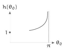
Fortunately, a thought experiment is cheap to im- prove: Replace the string with a massless steel rod. Balanced perfectly at \(θ_{0} = \pi\), the pendulum bob hangs upside down forever, so \(T(\pi) = \infty\) and \(h(\pi) = \infty\). Thus, \(h(\pi) > 1\) and \(h(0) = 1\). From these data, the most likely conjecture is that \(h\) increases monotonically with amplitude. Although h could first decrease and then increase, such twists and turns would be surprising behavior from such a clean differential equation. (For the behavior of h near θ\(_{0}\) = \pi, see Problem 3.34).
Problem 3.33 Small but nonzero amplitude
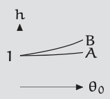
As the amplitude approaches π, the dimensionless period h diverges to infinity; at zero amplitude, \(h = 1\). But what about the derivative of \(h\)? At zero amplitude (\(θ_{0} = 0\)), does \(h(θ_{0})\) have zero slope (curve A) or positive slope (curve B)?
Problem 3.34 Nearly vertical release
| B | |
| \(10^{-1}\) | 2.791297 |
| \(10^{-2}\) | 4.255581 |
| \(10^{-3}\) | 5.721428 |
| \(10^{-4}\) | 7.187298 |
Imagine releasing the pendulum from almost vertical: an initial angle \(\pi − β\) with \(β\) tiny. As a function of \(β\), roughly how long does the pendulum take to rotate by a significant angle say, by 1 rad? Use that information to predict how \(h(θ_{0}\)) behaves when \(θ_{0} ≈ \pi\). Check and refine your conjectures using the tabulated values. Then predict \(h(\pi − 10^{−5}\)).
Moderate amplitudes: Applying Lumping
The conjecture that h increases monotonically was derived using the extremes of zero and vertical amplitude, so it should apply at intermediate amplitudes. Before taking that statement on faith, recall a proverb from arms-control negotiations: “Trust, but verify.”
At moderate (small but nonzero) amplitudes, does the period, or its dimensionless cousin \(h\), increase with amplitude?
In the zero-amplitude extreme, \(\sin θ\) is close to \(θ\). That approximation turned the nonlinear pendulum equation
\[\frac{d^{2}θ}{dt^{2}} + \frac{g}{l}\sin θ = 0 \label{3.43} \]
into the linear, ideal-spring equation in which the period is independent of amplitude.
At nonzero amplitude, however, \(θ\) and \(\sin θ\) differ and their difference affects the period. To account for the difference and predict the period, split \(\sin θ\) into the tractable factor \(θ\) and an adjustment factor \(f(θ)\). The resulting equation is
\[\frac{d^{2} \theta}{d t^{2}}+\frac{g}{l} \theta \underbrace{\frac{\sin \theta}{\theta}}_{f(\theta)}=0\label{3.44} \]
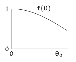
The nonconstant \(f(θ)\) encapsulates the nonlinearity of the pendulum equation. When \(θ\) is tiny, \(f(θ) ≈ 1\): The pendulum behaves like a linear, ideal-spring system. But when \(θ\) is large, \(f(θ)\) falls significantly below 1, making the ideal-spring approximation significantly inaccurate. As is often the case, a changing process is difficult to analyze for example, see the awful integrals in Problem 3.31. As a countermeasure, make a lumping approximation by replacing the changing \(f(θ)\) with a constant.
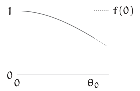
The simplest constant is f(0). Then the pendulum differential equation becomes
\[\frac{d^{2}θ}{dt^{2}} + \frac{g}{l}θ = 0. \label{3.45} \]
This equation is, again, the ideal-spring equation.
In this approximation, period does not depend on amplitude, so h = 1 for all amplitudes. For determining how the period of an unapproximated pendulum depends on amplitude, the \(f(θ) → f(0)\) lumping approximation discards too much information.
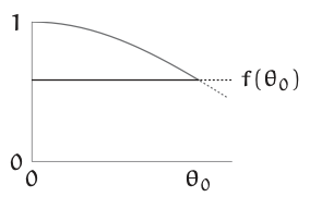
Therefore, replace \(f(θ)\) with the other extreme \(f(θ_{0}\)). Then the pendulum equation becomes
\[\frac{d^{2}θ}{dt^{2}} + \frac{g}{l}θf(θ_{0}) = 0. \label{3.46} \]
Is this Equation linear? What physical system does it describe ?
Because \(f(θ_{0}\)) is a constant, this equation is linear! It describes a zero amplitude pendulum on a planet with gravity \(g_{eff}\) that is slightly weaker than earth gravity as shown by the following slight regrouping:
\[\frac{d^{2} \theta}{d t^{2}}+\frac{\overbrace{g f\left(\theta_{0}\right)}^{g_{\text {eff }}}}{l} \theta=0 .\label{3.47} \]
Because the zero-amplitude pendulum has period \(T = 2π\sqrt{l/g}\), the zero amplitude, low-gravity pendulum has period
\[\mathrm{T}\left(\theta_{0}\right) \approx 2 \pi \sqrt{\frac{\mathrm{l}}{\mathrm{g}_{\mathrm{eff}}}}=2 \pi \sqrt{\frac{\mathrm{l}}{\mathrm{gf}\left(\theta_{0}\right)}} \label{3.48} \]
Using the dimensionless period h avoids writing the factors of \(2\pi\), \(l\), and \(g\), and it yields the simple prediction
\[h(θ_{0}) ≈ f(θ_{0})^{-1/2} = (\frac{sinθ_{0}}{θ_{0}})^{-1/2}. \label{3.49} \]
At moderate amplitudes the approximation closely follows the exact dimensionless period (dark curve). As a bonus, it also predicts \(h(\pi) = ∞\), so it agrees with the thought experiment of releasing the pendulum from upright (Section 3.5.3).
How much larger than the period at zero amplitude is the period at \(10^{◦}\) amplitude?
A \(10^o\) amplitude is roughly 0.17 rad, a moderate angle, so the approximate prediction for \(h\) can itself accurately be approximated using a Taylor series. The Taylor series for \(\sin θ\) begins \(θ − θ^{3}/6\), so
\[f(θ_{0} = \frac{\sinθ_{0}}{θ_{0}} ≈ 1 - \frac{θ_{0}^{2}}{6}. \label{3.50} \]
Then \(h(θ_{0})\), which is roughly \(f(θ_{0})^{-1/2}\), becomes
\[h(θ_{0}) ≈ (1 - \frac{θ_{0}^{2}}{6})^{-1/2}. \label{3.51} \]
Another Taylor series yields \((1 + x)^{-1/2} ≈ 1 − x/2\) (for small x). Therefore,
\[h(θ_{0}) ≈ 1 + \frac{θ_{0}^{2}}{12}. \label{3.52} \]
Restoring the dimensioned quantities gives the period itself.
\[T ≈ 2\pi\sqrt{\frac{l}{g}} (1 + \frac{θ_{0}^{2}}{12}). \label{3.53} \]
Compared to the period at zero amplitude, a \(10^{o}\) amplitude produces a fractional increase of roughly \(θ_{0}^{2}/12 ≈ 0.0025\) or 0.25%. Even at moderate amplitudes, the period is nearly independent of amplitude!
Use the preceding result for \(h(θ_{0})\) to check your conclusion in Problem 3.33 about the slope of \(h(θ_0)\) at \(θ_{0} = 0\).
Does our lumping approximation underestimate or overestimate the period?
The lumping approximation simplified the pendulum differential equation by replacing \(f(θ)\) with \(f(θ_{0}\)). Equivalently, it assumed that the mass always remained at the endpoints of the motion where \(|θ| = θ_{0}\). Instead, the pendulum spends much of its time at intermediate positions where \(|θ| < θ_{0}\) and \(f(θ) > f(θ_{0}\)). Therefore, the average f is greater than \(f(θ_{0}\)). Because h is inversely related to f \((h = f^{−1/2}\)), the \(f(θ) → f(θ_{0})\) lumping approximation overestimates h and the period.
The \(f(θ) → f(0)\) lumping approximation, which predicts \(T = 2\pi\sqrt{l/g}\), underestimates the period. Therefore, the true coefficient of the \(θ_{0}^{2}\) term in the period approximation
\[T ≈ 2\pi\sqrt{\frac{l}{g}}(1 + \frac{θ_{0}^{2}}{12}) \label{3.54} \]
lies between 0 and 1/12. A natural guess is that the coefficient lies halfway between these extremes namely, 1/24. However, the pendulum spends more time toward the extremes (where \(f(θ) = f(θ_{0})\)) than it spends near the equilibrium position (where \(f(θ) = f(0)\)). Therefore, the true coefficient is probably closer to 1/12 the prediction of the \(f(θ) → f(θ_{0}\)) approximation than it is to 0. An improved guess might be two-thirds of the way from 0 to 1/12, namely 1/18.
In comparison, a full successive-approximation solution of the pendulum differential equation gives the following period [13, 33]:
\[\mathrm{T}=2 \pi \sqrt{\frac{l}{\mathrm{~g}}}\left(1+\frac{1}{16} \theta_{0}^{2}+\frac{11}{3072} \theta_{0}^{4}+\cdots\right)\label{3.55} \]
Our educated guess of 1/18 is very close to the true coefficient of 1/16!