1.30: Standard Deviation

Last updated
Save as PDF

Page ID: 56869

$ \newcommand{\vecs}[1]{\overset { \scriptstyle \rightharpoonup} {\mathbf{#1}} } $ $ \newcommand{\vecd}[1]{\overset{-\!-\!\rightharpoonup}{\vphantom{a}\smash {#1}}} $$\newcommand{\id}{\mathrm{id}}$ $ \newcommand{\Span}{\mathrm{span}}$ $ \newcommand{\kernel}{\mathrm{null}\,}$ $ \newcommand{\range}{\mathrm{range}\,}$ $ \newcommand{\RealPart}{\mathrm{Re}}$ $ \newcommand{\ImaginaryPart}{\mathrm{Im}}$ $ \newcommand{\Argument}{\mathrm{Arg}}$ $ \newcommand{\norm}[1]{\| #1 \|}$ $ \newcommand{\inner}[2]{\langle #1, #2 \rangle}$ $ \newcommand{\Span}{\mathrm{span}}$ $\newcommand{\id}{\mathrm{id}}$ $ \newcommand{\Span}{\mathrm{span}}$ $ \newcommand{\kernel}{\mathrm{null}\,}$ $ \newcommand{\range}{\mathrm{range}\,}$ $ \newcommand{\RealPart}{\mathrm{Re}}$ $ \newcommand{\ImaginaryPart}{\mathrm{Im}}$ $ \newcommand{\Argument}{\mathrm{Arg}}$ $ \newcommand{\norm}[1]{\| #1 \|}$ $ \newcommand{\inner}[2]{\langle #1, #2 \rangle}$ $ \newcommand{\Span}{\mathrm{span}}$$\newcommand{\AA}{\unicode[.8,0]{x212B}}$

This topic requires a leap of faith. It is one of the rare times when this textbook will say “don’t worry about why it’s true; just accept it.”

A normal distribution, often referred to as a bell curve, is symmetrical on the left and right, with the mean, median, and mode being the value in the center. There are lots of data values near the center, then fewer and fewer as the values get further from the center. A normal distribution describes the data in many real-world situations: heights of people, weights of people, errors in measurement, scores on standardized tests (IQ, SAT, ACT)…

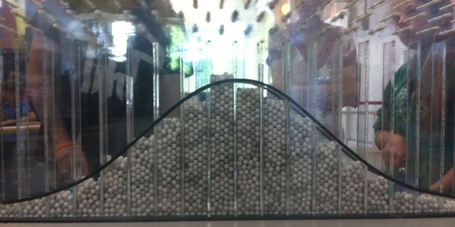
One of the best ways to demonstrate the normal distribution is to drop balls through a board of evenly spaced pegs, as shown here.^[1] Each time a ball hits a peg, it has a fifty-fifty chance of going left or right. For most balls, the number of lefts and rights are roughly equal, and the ball lands near the center. Only a few balls have an extremely lopsided number of lefts and rights, so there are not many balls at either end. As you can see, the distribution is not perfect, but it is approximated by the normal curve drawn on the glass.

$science museum demonstration showing balls dropped forming a bell curve$

The standard deviation is a measure of the spread of the data: data with lots of numbers close to the mean has a smaller standard deviation, and data with numbers spaced further from the mean has a larger standard deviation. (In this textbook, you will be given the value of the standard deviation of the data and will never need to calculate it.) The standard deviation is a measuring stick for a particular set of data.

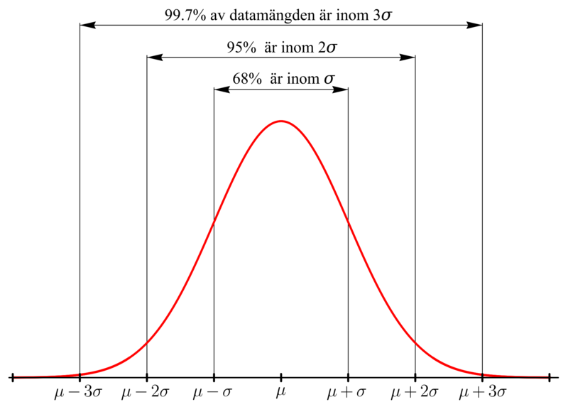
In a normal distribution…

roughly $68\%$ of the numbers are within $1$ standard deviation above or below the mean
roughly $95\%$ of the numbers are within $2$ standard deviations above or below the mean
roughly $99.7\%$ of the numbers are within $3$ standard deviations above or below the mean

This 68-95-99.7 rule is called an empirical rule because it is based on observation rather than some formula. Nobody discovered a calculation to figure out the numbers $68\%$, $95\%$, and $99.7\%$ until after the fact. Instead, statisticians looked at lots of different examples of normally distributed data and said “Mon Dieu, it appears that if you count up the data values that are within one standard deviation above or below the mean, you have about $68\%$ of the data!” and so on.^[2]

The following image is in Swedish, but you can probably decipher it because math is an international language.

$a bell curve showing the 68-95-99.7 rule: matching vertical lines one unit to the left and right of the center include 68 percent of the data, matching vertical lines two units to the left and right of the center include 95 percent of the data, and matching vertical lines three units to the left and right of the center include 99.7 percent of the data.$

Let’s go back to the ball-dropping experiment, and let’s assume that the standard deviation is three columns wide.^[3] In the picture below, the green line marks the center of the distribution.

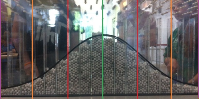
$science museum demonstration showing balls dropped forming a bell curve, with vertical lines drawn to show the standard deviations$

First, the two red lines are each three columns away from the center, which is one standard deviation above and below the center, so about 68% of the balls will land between the red lines.

Next, the two orange lines are another three columns farther away from the center, which is six columns or two standard deviations above and below the center, so about 95% of the balls will land between the orange lines.

And finally, the two purple lines are another three columns farther away from the center, which is nine columns or three standard deviations above and below the center, so about 99.7% of the balls will land between the purple lines. We can expect that $997$ out of $1,000$ balls will land between the purple lines, leaving only $3$ out of $1,000$ landing beyond the purple lines on either end.

Here are Damian Lillard’s game results for points scored, in increasing order, for the $80$ games he played in the 2018-19 NBA season.^[4] This is broken up into eight rows of ten numbers each, and this is a total of $2,069$ points.

$11$, $13$, $13$, $13$, $14$, $14$, $15$, $15$, $15$, $16$,
$16$, $16$, $17$, $17$, $17$, $18$, $18$, $19$, $19$, $20$,
$20$, $20$, $20$, $20$, $21$, $21$, $22$, $22$, $23$, $23$,
$23$, $23$, $24$, $24$, $24$, $24$, $24$, $24$, $24$, $24$,
$25$, $25$, $25$, $26$, $26$, $26$, $28$, $28$, $28$, $29$,
$29$, $29$, $29$, $30$, $30$, $30$, $30$, $30$, $31$, $31$,
$33$, $33$, $33$, $33$, $33$, $33$, $34$, $34$, $34$, $35$,
$36$, $36$, $37$, $39$, $40$, $40$, $41$, $41$, $42$, $51$

Exercises $\PageIndex{1}$

This is a review of mean, median, and mode; you’ll need to know the mean in order to complete the standard deviation exercises that follow.

1. What is the mean of the data? (Round to the nearest tenth.)

2. What is the median of the data?

3. What is the mode of the data?

4. Do any of the mean, median, or mode seems misleading, or do all three seem to represent the data fairly well?

Answer

1. $25.9$ points

2. $24.5$ points

3. $24$ points (which occurred eight times)

4. all three seem to represent the typical number of points scored; the mean is a bit high because there are no extremely low values but there are a few high values that pull the mean upwards.

Here is a histogram of the data, arbitrarily grouped in seven equally-spaced intervals. It shows that the data roughly follows a bell-shaped curve, somewhat truncated on the left and with an outlier on the right.

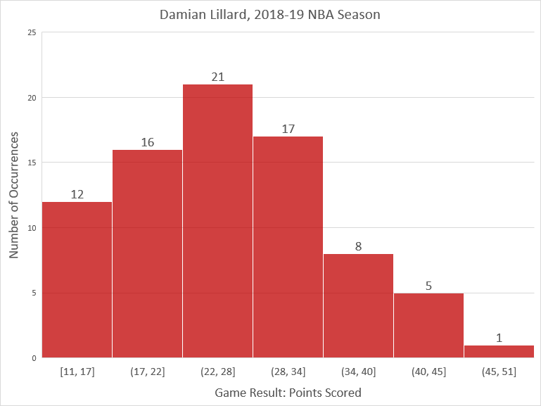
$a histogram or bar graph showing 12 scores between 11 and 17, 16 scores above 17 and up to 22, 21 scores above 22 and up to 28, 17 scores above 28 and up to 34, 8 scores above 34 and up to 40, 5 scores above 40 and up to 45, and 1 score above 45 and up to 51.$

If we enter the data into a spreadsheet program such as Microsoft Excel or Google Sheets, we can quickly find that the standard deviation is $8.2$ points.

Based on the empirical rule, we should expect approximately $68\%$ of the results to be within $8.2$ points above and below the mean.

Exercises $\PageIndex{1}$

5. Determine the range of points scored that are within one standard deviation of the mean.

6. How many of the $80$ game results are within one standard deviation of the mean?

7. Is the previous answer close to $68\%$ of the total number of game results?

Answer

5. $17.7$ to $34.1$ points

6. $54$ of the $80$ game results

7. yes; $54\div80=67.5\%$

And we should expect approximately $95\%$ of the results to be within $2\cdot8.2=16.4$ points above and below the mean.

Exercises $\PageIndex{1}$

8. Determine the range of points scored that are within two standard deviations of the mean.

9. How many of the $80$ game results are within two standard deviations of the mean?

10. Is the previous answer close to $95\%$ of the total number of game results?

Answer

8. $9.5$ to $42.3$ points

9. $79$ of the $80$ game results

10. sort of close but not really; $79\div80=98.75\%$

And we should expect approximately $99.7\%$ of the results to be within $3\cdot8.2=24.6$ points above and below the mean.

Exercises $\PageIndex{1}$

11. Determine the range of points scored that are within three standard deviations of the mean.

12. How many of the $80$ game results are within three standard deviations of the mean?

13. Is the previous answer close to $99.7\%$ of the total number of game results?

Answer

11. $1.3$ to $50.5$ points

12. $79$ of the $80$ game results, again

13. yes, this is pretty close; $79\div80=98.75\%$

Notice that we could think about the standard deviations like a measurement error or tolerance: the mean $\pm8.2$, the mean $\pm16.4$, the mean $\pm24.6$…

Exercises $\PageIndex{1}$

For U.S. females, the average height is around $63.5$ inches ($5$ ft $3.5$ in) and the standard deviation is $3$ inches. Use the empirical rule to fill in the blanks.

14. About $68\%$ of the women should be between _______ and _______ inches tall.

15. About $95\%$ of the women should be between _______ and _______ inches tall.

16. About $99.7\%$ of the women should be between _______ and _______ inches tall.

For U.S. males, the average height is around $69.5$ inches ($5$ ft $9.5$ in) and the standard deviation is $3$ inches. Use the empirical rule to fill in the blanks.

17. About $68\%$ of the men should be between _______ and _______ inches tall.

18. About $95\%$ of the men should be between _______ and _______ inches tall.

19. About $99.7\%$ of the men should be between _______ and _______ inches tall.

Answer

14. $60.5$; $66.5$

15. $57.5$; $69.5$

16. $54.5$; $72.5$

17. $66.5$; $72.5$

18. $63.5$; $75.5$

19. $60.5$; $78.5$

This graph at https://tall.life/height-percentile-calculator-age-country/ shows that, because the standard deviations are equal, the two bell curves have essentially the same shape but the women’s graph is centered six inches below the men’s.

Exercises $\PageIndex{1}$

Around $16\%$ of U.S. males in their forties weigh less than $160$ lb and $16\%$ weigh more than $230$ lb.^[5] Assume a normal distribution.

20. What percent of U.S. males weigh between $160$ lb and $230$ lb?

21. What is the average weight? (Hint: think about symmetry.)

22. What is the standard deviation? (Hint: You have to work backwards to figure this out, but the math isn’t complicated.)

23. Based on the empirical rule, about $95\%$ of the men should weigh between _______ and _______ pounds.

Answer

20. $68\%$ because $100\%-(16\%+16\%)=68\%$

21. $195$ lb because this is halfway between $160$ and $230$ lb

22. $35$ lb because $195-35$ lb and $195+35$ lb encompasses $68\%$ of the data

23. $125$; $265$

If you are asked only one question about the empirical rule instead of three in a row ($68\%$, $95\%$, $99.7\%$), you will most likely be asked about the $95\%$. This is related to the “$95\%$ confidence interval” that is often mentioned in relation to statistics. For example, the margin of error for a poll is usually close to two standard deviations.^[6]

Let’s finish up by comparing the performance of three NFL teams since the turn of the century.

The numbers of regular-season games won by the New England Patriots each NFL season from 2001-19:^[7]

year	wins
2001	$11$
2002	$9$
2003	$14$
2004	$14$
2005	$10$
2006	$12$
2007	$16$
2008	$11$
2009	$10$
2010	$14$
2011	$13$
2012	$12$
2013	$12$
2014	$12$
2015	$12$
2016	$14$
2017	$13$
2018	$11$
2019	$12$

Exercises $\PageIndex{1}$

For the Patriots, the mean number of wins is $12.2$, and a spreadsheet tells us that the standard deviation is $1.7$ wins.

24. There is a $95\%$ chance of the Patriots winning between _______ and _______ games in a season.

25. In 2020, the Patriots won $7$ games. Could you have predicted that based on the data? How many standard deviations from the mean is this number of wins?

Answer

24. $8.8$; $15.6$

25. You would not have predicted this from the data because it is more than two standard deviations below the mean, so there would be a roughly $2.5\%$ chance of this happening randomly. In fact, $(12.2-7)\div1.7$ is slightly larger than $3$, so this is more than three standard deviations below the mean, making it even more unlikely. (You might have predicted that the Patriots would get worse when Tom Brady left them for Tampa Bay, but you wouldn’t have predicted only $7$ wins based on the previous nineteen years of data.)

The numbers of regular-season games won by the Buffalo Bills each NFL season from 2001-19:^[8]

year	wins
2001	$3$
2002	$8$
2003	$6$
2004	$9$
2005	$5$
2006	$7$
2007	$7$
2008	$7$
2009	$6$
2010	$4$
2011	$6$
2012	$6$
2013	$6$
2014	$9$
2015	$8$
2016	$7$
2017	$9$
2018	$6$
2019	$10$

Exercises $\PageIndex{1}$

For the Bills, the mean number of wins is $6.8$, and a spreadsheet tells us that the standard deviation is $1.7$ wins.

26. There is a $95\%$ chance of the Bills winning between _______ and _______ games in a season.

27. In 2020, the Bills won $13$ games. Could you have predicted that based on the data? How many standard deviations from the mean is this number of wins?

Answer

26. $3.4$; $10.2$

27. You would not predict this from the data because it is more than two standard deviations above the mean, so there would be a roughly $2.5\%$ chance of this happening randomly. In fact, $(13-6.8)\div1.7\approx3.6$, so this is more than three standard deviations above the mean, making it even more unlikely. This increased win total is partly due to external forces (i.e., the Patriots becoming weaker and losing two games to the Bills) but even $11$ wins would have been a bold prediction, let alone $13$.

The numbers of regular-season games won by the Denver Broncos each NFL season from 2001-19:^[9]

year	wins
2001	$8$
2002	$9$
2003	$10$
2004	$10$
2005	$13$
2006	$9$
2007	$7$
2008	$8$
2009	$8$
2010	$4$
2011	$8$
2012	$13$
2013	$13$
2014	$12$
2015	$12$
2016	$9$
2017	$5$
2018	$6$
2019	$7$

Exercises $\PageIndex{1}$

For the Broncos, the mean number of wins is $9.1$, and a spreadsheet tells us that the standard deviation is $2.6$ wins.

28. There is a $95\%$ chance of the Broncos winning between _______ and _______ games in a season.

29. In 2020, the Broncos won $5$ games. Could you have predicted that based on the data? How many standard deviations from the mean is this number of wins?

Answer

28. $3.9$; $14.3$

29. The trouble with making predictions about the Broncos is that their standard deviation is so large. You could choose any number between $4$ and $14$ wins and be within the $95\%$ interval. $(9.1-5)\div2.6\approx1.6$, so this is around $1.6$ standard deviations below the mean, which makes it not very unusual. Whereas the Patriots and Bills are more consistent, the Broncos’ win totals fluctuate quite a bit and are therefore more unpredictable.

The Plinko game on The Price Is Right is the best-known example of this; here's a clip of Snoop Dogg helping a contestant win some money. ↵
Confession: This paragraph gives you the general idea of how these ideas developed but may not be perfectly historically accurate. ↵
I eyeballed it and it seemed like a reasonable assumption. ↵
Source: https://www.basketball-reference.com/players/l/lillada01/gamelog/2019 ↵
Source: https://www.google.com/url?sa=t&rct=j&q=&esrc=s&source=web&cd=17&ved=2ahUKEwjm-d-whavhAhWCFXwKHQxMDz4QFjAQegQIARAC&url=https%3A%2F%2Fwww2.census.gov%2Flibrary%2Fpublications%2F2010%2Fcompendia%2Fstatab%2F130ed%2Ftables%2F11s0205.pdf&usg=AOvVaw1DFDbil78g-qXbIgK6JirW ↵
Source: https://en.Wikipedia.org/wiki/Standard_deviation ↵
Source: https://www.pro-football-reference.com/teams/nwe/index.htm ↵
Source: https://www.pro-football-reference.com/teams/buf/index.htm ↵
Source: https://www.pro-football-reference.com/teams/den/index.htm ↵

Exercises \(\PageIndex{1}\)

Exercises \(\PageIndex{1}\)

Exercises \(\PageIndex{1}\)

Exercises \(\PageIndex{1}\)

Exercises \(\PageIndex{1}\)

Exercises \(\PageIndex{1}\)

Exercises \(\PageIndex{1}\)

Exercises \(\PageIndex{1}\)

Exercises \(\PageIndex{1}\)