1.5: Properties of Continuous Functions

Suppose \(f\) is continuous at the real number \(c\) and \(k\) is any fixed real number. If we let \(h(x)=k g(x),\) then, for any infinitesimal \(\epsilon\),

\[h(c+\epsilon)-h(c)=k f(c+\epsilon)-k f(c)=k(f(c+\epsilon)-f(c))\] is an infinitesimal since, by assumption, \(f(c+\epsilon)-f(c)\) is an infinitesimal. Hence \(h(c+\epsilon) \simeq h(c)\).

Theorem \(\PageIndex{1}\)

If \(f\) is continuous at \(c\) and \(k\) is any fixed real number, then the function \(h(x)=k f(x)\) is also continuous at \(c .\)

Example \(\PageIndex{1}\)

We have seen that \(f(x)=x^{2}\) is continuous on \((-\infty, \infty) .\) It now follows that, for example, \(g(x)=5 x^{2}\) is also continuous on \((-\infty, \infty)\).

Suppose that both \(f\) and \(g\) are continuous at the real number \(c\) and we let \(s(x)=f(x)+g(x) .\) If \(\epsilon\) is any infinitesimal, then \[s(c+\epsilon)=f(c+\epsilon)+g(c+\epsilon) \simeq f(c)+g(c)=s(c) ,\] and so \(s\) is also continuous at \(c .\)

Theorem \(\PageIndex{2}\)

If \(f\) and \(g\) are both continuous at \(c,\) then the function

\[s(x)=f(x)+g(x)\] is also continuous at \(c .\)

Example \(\PageIndex{2}\)

Since

\[(x+\epsilon)^{3}=x^{3}+3 x^{2} \epsilon+3 x \epsilon^{2}+\epsilon^{3} \simeq x^{3}\] for any real number \(x\) and any infinitesimal \(\epsilon,\) it follows that \(g(x)=x^{3}\) is continuous on \((-\infty, \infty) .\) From the previous theorems, it then follows that \[h(x)=5 x^{2}+3 x^{3}\] is continuous on \((-\infty, \infty)\). Again, suppose \(f\) and \(g\) are both continuous at \(c\) and let \(p(x)=f(x) g(x)\). Then, for any infinitesimal \(\epsilon\), \[\begin{aligned} p(c+\epsilon)-s(c) &=f(c+\epsilon) g(c+\epsilon)-f(c) g(c) \\[12pt] &=f(c+\epsilon) g(c+\epsilon)-f(c) g(c+\epsilon)+f(c) g(c+\epsilon)-f(c) g(c) \\[12pt] &=g(c+\epsilon)(f(c+\epsilon)-f(c))+f(c)(g(c+\epsilon)-g(c)), \end{aligned}\] which is infinitesimal since both \(f(c+\epsilon)-f(c)\) and \(g(c+\epsilon)-g(c)\) are. Hence \(p\) is continuous at \(c .\)

Theorem \(\PageIndex{3}\)

If \(f\) and \(g\) are both continuous at \(c,\) then the function

\[p(x)=f(x) g(x)\] is also continuous at \(c .\) Finally, suppose \(f\) and \(g\) are continuous at \(c\) and \(g(c) \neq 0 .\) Let \(q(x)=\frac{f(x)}{g(x)}\). Then, for any infinitesimal \(\epsilon,\) \[\begin{aligned} q(c+\epsilon)-q(c) &=\frac{f(c+\epsilon)}{g(c+\epsilon)}-\frac{f(c)}{g(c)} \\[12pt] &=\frac{f(c+\epsilon) g(c)-f(c) g(c+\epsilon)}{g(c+\epsilon) g(c)} \\[12pt] &=\frac{f(c+\epsilon) g(c)-f(c) g(c)+f(c) g(c)-f(c) g(c+\epsilon)}{g(c+\epsilon) g(c)} \\[12pt] &=\frac{g(c)(f(c+\epsilon)-f(c))-f(c)(g(c+\epsilon)-g(c))}{g(c+\epsilon) g(c)}, \end{aligned}\] which is infinitesimal since both \(f(c+\epsilon)-f(c)\) and \(g(c+\epsilon)-g(c)\) are infinitesimals, and \(g(c) g(c+\epsilon)\) is not an infinitesimal. Hence \(q\) is continuous at \(c .\)

Theorem \(\PageIndex{4}\)

If \(f\) and \(g\) are both continuous at \(c\) and \(g(c) \neq 0,\) then the function

\[q(x)=\frac{f(x)}{g(x)}\] is continuous at \(c .\)

Exercise \(\PageIndex{1}\)

Explain why

\[f(x)=\frac{3 x+4}{x^{2}+1}\] is continuous on \((-\infty, \infty)\).

Polynomials and Rational Functions

It is now possible to identify two important classes of continuous functions. First, every constant function is continuous: indeed, if \(f(x)=k\) for all real values \(x,\) and \(k\) is any real constant, then for any infinitesimal \(\epsilon\),

\[f(x+\epsilon)=k=f(x) .\] Next, the function \(f(x)=x\) is continuous for all real \(x\) since, for any infinitesimal \(\epsilon\), \[f(x+\epsilon)=x+\epsilon \simeq x=f(x) .\] Since the product of continuous functions is continuous, it now follows that, for any nonnegative integer \(n, g(x)=x^{n}\) is continuous on \((-\infty, \infty)\) since it is a constant function if \(n=0\) and a product of \(f(x)=x\) by itself \(n\) times otherwise. From this it follows (since constant multiples of continuous functions are again continuous) that all monomials, that is, functions of the form \(f(x)=a x^{n},\) where \(a\) is a fixed real constant and \(n\) is a nonnegative integer, are continuous. Now a polynomial is a function of the form \[P(x)=a_{0}+a_{1} x+a_{2} x^{2}+\cdots+a_{n} x^{n} ,\] where \(a_{0}, a_{1}, \ldots, a_{n}\) are real constants and \(n\) is a nonnegative integer. That is, a polynomial is a sum of monomials. since sums of continuous functions are continuous, we now have the following fundamental result.

Theorem \(\PageIndex{5}\)

If \(P\) is a polynomial, then \(P\) is continuous on \((\infty, \infty)\).

Example \(\PageIndex{3}\)

The function

\[f(x)=32+14 x^{5}-6 x^{7}+\pi x^{14}\] is continuous on \((-\infty, \infty)\). A rational function is a ratio of polynomials. That is, if \(P(x)\) and \(Q(x)\) are polynomials, then \[R(x)=\frac{P(x)}{Q(x)}\] is a rational function. since ratios of continuous functions are continuous, we have the following.

Theorem \(\PageIndex{6}\)

If \(R\) is rational function, then \(R\) is continuous at every point in its domain.

Example \(\PageIndex{4}\)

If

\[f(x)=\frac{3 x-4}{x^{2}-1} ,\] then \(f\) is a rational function defined for all real \(x\) except \(x=-1\) and \(x=1 .\) Thus \(f\) is continuous on the intervals \((-\infty,-1),(-1,1),\) and \((1, \infty) .\)

Exercise \(\PageIndex{2}\)

Find the intervals on which

\[f(x)=\frac{3 x^{2}-1}{x^{3}+1}\] is continuous.

Answer

\((-\infty,-1)\) and \((-1, \infty)\)

Trigonometric Functions

Recall that if \(t\) is a real number and \((a, b)\) is the point in the plane found by traversing the unit circle \(x^{2}+y^{2}=1\) a distance \(|t|\) from \((1,0),\) in the counterclockwise direction if \(t \geq 0\) and in the clockwise direction otherwise, then

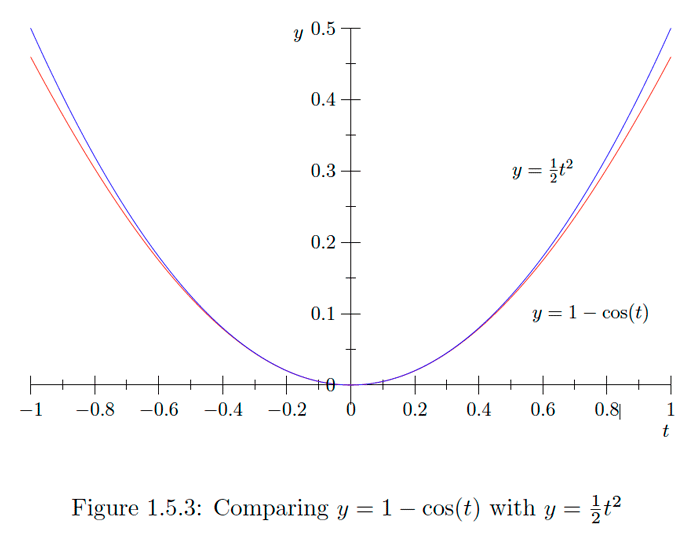
\[a=\cos (t)\] \[b=\sin (t) .\] Note that for \(0<t<\pi\), as in Figure \(1.5 .1, t\) is greater than the length of the line segment from \(A=(1,0)\) to \(B=(\cos (t), \sin (t)) .\) Now the segment from \(A\) to \(B\) is the hypotenuse of the right triangle with vertices at \(A, B,\) and \(C=(\cos (t), 0) . \text { since the distance from } C \text { to } A \text { is } 1-\cos (t))\) and the distance from \(B\) to \(C\) is \(\sin (t),\) it follows from the Pythagorean theorem that \[\begin{aligned} t^{2} &>(1-\cos (t))^{2}+\sin ^{2}(t) \\ &=1-2 \cos (t)+\cos ^{2}(t)+\sin ^{2}(t) \\ &=2-2 \cos (t) . \end{aligned}\] A similar diagram reveals the same result for \(-\pi<t<0 .\) Moreover, both \(t^{2}\) and \(2-2 \cos (t)\) are 0 when \(t=0,\) so we have \(t^{2} \geq 2-2 \cos (t)\) for all \(-\pi<t<\pi\). Additionally, \(0 \leq 2-2 \cos (t) \leq 4 \text { for all } t \text { (since }-1 \leq \cos (t) \leq 1 \text { for all } t)\), so certainly \(t^{2}>2-2 \cos (t)\) whenever \(|t|>2 .\) Hence we have shown that \[0 \leq 2-2 \cos (t) \leq t^{2}\]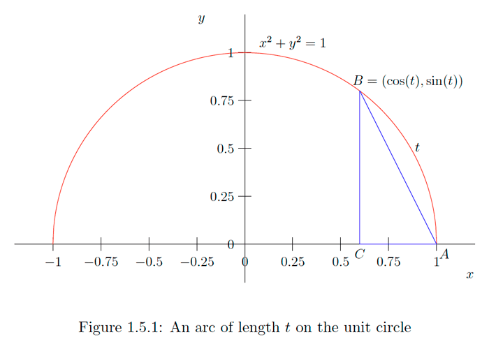

\[\text { for all values of } t . \text { Equivalently, }\] for all values of \(t .\) Equivalently, \[0 \leq 1-\cos (t) \leq \frac{1}{2} t^{2}\] Solving for \(\cos (t),\) we may also write this as

\[1-\frac{t^{2}}{2} \leq \cos (t) \leq 1\]

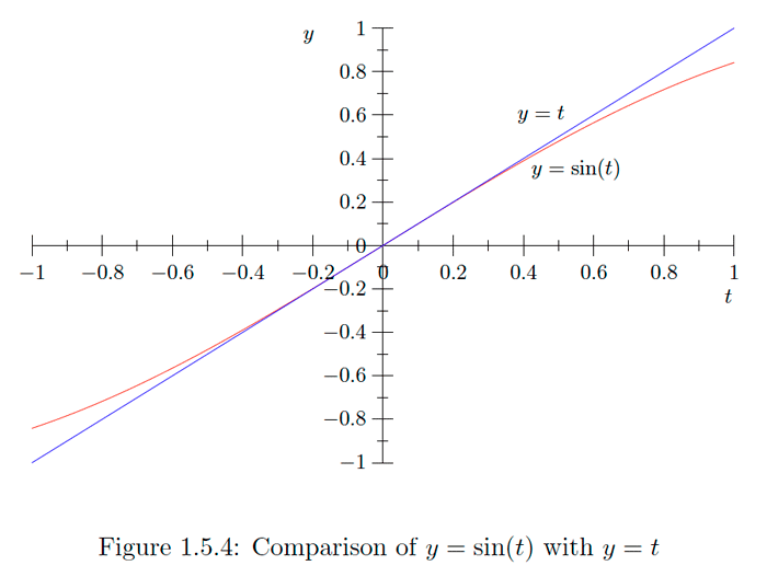
for all \(t .\) In particular, if \(\epsilon\) is an infinitesimal, then \[1-\frac{\epsilon^{2}}{2} \leq \cos (\epsilon) \leq 1\] implies that \[\cos (0+\epsilon)=\cos (\epsilon) \simeq 1=\cos (0) .\] That is, the function \(f(t)=\cos (t)\) is continuous at \(t=0 .\) Moreover, since \(0 \leq 1+\cos (t) \leq 2\) for all \(t\), \[\begin{aligned} \sin ^{2}(t) &=1-\cos ^{2}(t) \\ &=(1-\cos (t))(1+\cos (t)) \\ & \leq \frac{t^{2}}{2}(1+\cos (t)) \\ & \leq t^{2} , \end{aligned}\] from which it follows that \[|\sin (t)| \leq|t|\] for any value of \(t .\) In particular, for any infinitesimal \(\epsilon\), \[|\sin (0+\epsilon)|=|\sin (\epsilon)| \leq \epsilon ,\] from which it follows that \[\sin (\epsilon) \simeq 0=\sin (0) .\] That is, the function \(g(t)=\sin (t)\) is continuous at \(t=0\). Using the angle addition formulas for sine and cosine, we see that, for any real number \(t\) and infinitesimal \(\epsilon\), \[\cos (t+\epsilon)=\cos (t) \cos (\epsilon)-\sin (t) \sin (\epsilon) \simeq \cos (t)\] and \[\sin (t+\epsilon)=\sin (t) \cos (\epsilon)+\cos (t) \sin (\epsilon) \simeq \sin (t) ,\] since \(\cos (\epsilon) \simeq 1\) and \(\sin (\epsilon)\) is an infinitesimal. Hence we have the following result.

Theorem \(\PageIndex{7}\)

The functions \(f(t)=\cos (t)\) and \(g(t)=\sin (t)\) are continuous on \((-\infty, \infty)\).

The following theorem now follows from our earlier results about continuous functions.

Theorem \(\PageIndex{8}\)

The following functions are continuous at each point in their respective domains:

\[\tan (t)=\frac{\sin (t)}{\cos (t)} ,\] \[\cot (t)=\frac{\cos (t)}{\sin (t)} ,\] \[\sec (t)=\frac{1}{\cos (t)} ,\] \[\csc (t)=\frac{1}{\sin (t)} ,\] With a little more geometry, we may improve upon the inequalities in \((1.5 .13)\) and \((1.5 .18) .\) Consider an angle \(0<t<\frac{\pi}{2},\) let \(A=(1,0)\) and \(B=(\cos (t), \sin (t))\) as above, and let \(D\) be the point of intersection of the lines tangent to the circle \(\left.x^{2}+y^{2}=1 \text { at } A \text { and } B \text { (see Figure } 1.5 .2\right) .\) Note that the triangle with vertices at \(A, B,\) and \(D\) is isosceles with base of length \(\sqrt{2(1-\cos (t))}\) (as derived above) and base angles \(\frac{t}{2} .\) Moreover, the sum of the lengths of the two legs exceeds \(t\). since each leg is of length \[\frac{\frac{1}{2} \sqrt{2(1-\cos (t))}}{\cos \left(\frac{t}{2}\right)} ,\]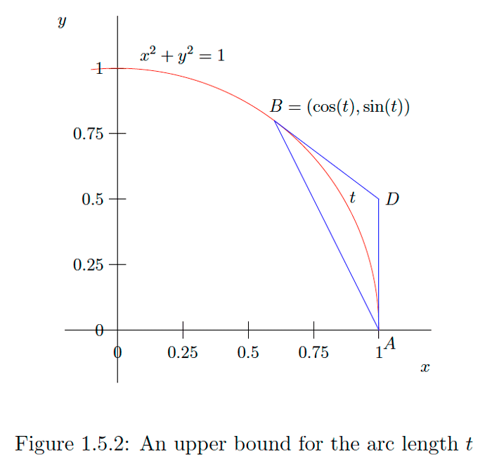

it follows that \[t<\frac{\sqrt{2(1-\cos (t))}}{\cos \left(\frac{t}{2}\right)} .\] Moreover, both sides of this inequality are 0 when \(t=0\) and we could derive the same inequality for \(-\frac{\pi}{2}<t<0,\) so we have \[t \leq \frac{\sqrt{2(1-\cos (t))}}{\cos \left(\frac{t}{2}\right)}\] for all \(-\frac{\pi}{2}<t<\frac{\pi}{2} .\) It now follows that \[\frac{1}{2} t^{2} \leq \frac{1-\cos (t)}{\cos ^{2}\left(\frac{t}{2}\right)}=\frac{2(1-\cos (t))}{1+\cos (t)}\] for all \(-\frac{\pi}{2}<t<\frac{\pi}{2},\) where we have used the half-angle identity \[\cos ^{2}\left(\frac{t}{2}\right)=\frac{1+\cos (t)}{2} .\] Combining \((1.5 .30)\) with \((1.5 .13),\) we have \[1-\cos (t) \leq \frac{1}{2} t^{2} \leq \frac{2(1-\cos (t))}{1+\cos (t)} ,\] from which we obtain, for all \(-\frac{\pi}{2}<t<\frac{\pi}{2}\), \[\frac{1+\cos (t)}{2} \leq \frac{1-\cos (t)}{\frac{1}{2} t^{2}} \leq 1 .\]

Now if \(\epsilon\) is an infinitesimal, then \(1+\cos (\epsilon) \simeq 2,\) and so \[\frac{1+\cos (\epsilon)}{2} \simeq 1 .\] Hence, substituting \(t=\epsilon\) in \((1.5 .33),\) we have \[\frac{1-\cos (\epsilon)}{\frac{1}{2} \epsilon^{2}} \simeq 1 .\] Moreover, we then have \[\frac{\sin ^{2}(\epsilon)}{\epsilon^{2}}=\frac{1-\cos ^{2}(\epsilon)}{\epsilon^{2}}=\frac{1-\cos (\epsilon)}{\epsilon^{2}}(1+\cos (t)) \simeq \frac{1}{2}(2)=1 .\] Since \(\epsilon\) and \(\sin (\epsilon)\) have the same sign, it follows that \[\frac{\sin (\epsilon)}{\epsilon} \simeq 1 .\] For real numbers \(t,(1.5 .34)\) and \((1.5 .36)\) say that, for small values of \(t\), \[\cos (t) \approx 1-\frac{t^{2}}{2}\] and \[\sin (t) \approx t .\] Figures 1.5 .3 and 1.5 .4 graphically display the comparisons in \((1.5 .37)\) and \((1.5 .38) .\)

Example \(\PageIndex{5}\)

For a numerical comparison, note that for \(t=0.1, \cos (t)= 0.9950042,\) compared to \(1-\frac{t^{2}}{2}=0.995,\) and \(\sin (t)=0.0998334,\) compared to \(t=0.1\)

Exercise \(\PageIndex{3}\)

Verify that the triangle with vertices at \(A, B,\) and \(D\) in Figure 1.5 .2 is an isosceles triangle with base angles of \(\frac{t}{2}\) at \(A\) and \(B\).

Exercise \(\PageIndex{4}\)

Verify the half-angle formula,

\[\cos (\theta)=\frac{1}{2}(1+\cos (2 \theta)) ,\] for any angle \(\theta,\) using the identities \(\cos (2 \theta)=\cos ^{2}(\theta)-\sin ^{2}(\theta)\) (a consequence of the addition formula) and \(\sin ^{2}(\theta)+\cos ^{2}(\theta)=1\).

Compositions

Given functions \(f\) and \(g,\) we call the function

\[f \circ g(x)=f(g(x))\] the composition of \(f\) with \(g .\) If \(g\) is continuous at a real number \(c, f\) is continuous at \(g(c),\) and \(\epsilon\) is an infinitesimal, then \[f \circ g(c+\epsilon)=f(g(c+\epsilon)) \simeq f(g(c))\] since \(g(c+\epsilon) \simeq g(c)\).

Theorem \(\PageIndex{9}\)

If \(g\) is continuous at \(c\) and \(f\) is continuous at \(g(c),\) then \(f \circ g\) is continuous at \(c .\)

Example \(\PageIndex{6}\)

Since \(f(t)=\sin (t)\) is continuous for all \(t\) and

\[g(t)=\frac{3 t^{2}+1}{4 t-8}\] is continuous at all real numbers except \(t=2,\) it follows that \[h(t)=\sin \left(\frac{3 t^{2}+1}{4 t-8}\right)\] is continuous on the intervals \((-\infty, 2)\) and \((2, \infty)\). Note that if \(f(x)=\sqrt{x}\) and \(\epsilon\) is an infinitesimal, then, for any \(x \neq 0\), \[\begin{aligned} f(x+\epsilon)-f(x) &=\sqrt{x+\epsilon}-\sqrt{x} \\ &=(\sqrt{x+\epsilon}-\sqrt{x})\left(\frac{\sqrt{x+\epsilon}+\sqrt{x}}{\sqrt{x+\epsilon}+\sqrt{x}}\right) \\ &=\frac{x+\epsilon-x}{\sqrt{x+\epsilon}+\sqrt{x}} \\ &=\frac{\epsilon}{\sqrt{x+\epsilon}+\sqrt{x}} , \end{aligned}\] which is infinitesimal. Hence \(f\) is continuous on \((0, \infty) .\) Moreover, if \(\epsilon\) is a positive infinitesimal, then \(\sqrt{\epsilon}\) must be an infinitesimal (since if \(a=\sqrt{\epsilon}\) is not an infinitesimal, then \(a^{2}=\epsilon\) is not an infinitesimal). Hence \[f(0+\epsilon)=\sqrt{\epsilon} \simeq 0=f(0) .\] Thus \(f\) is continuous at \(0,\) and so \(f(x)=\sqrt{x}\) is continuous on \([0, \infty)\).

Theorem \(\PageIndex{10}\)

The function \(f(x)=\sqrt{x}\) is continuous on \([0, \infty)\).

Example \(\PageIndex{7}\)

It now follows that \(f(x)=\sqrt{4 x-2}\) is continuous everywhere it is defined, namely, on \([2, \infty)\).

Exercise \(\PageIndex{5}\)

Find the interval or intervals on which \(f(x)=\sin \left(\frac{1}{x}\right)\) is continuous.

Answer

\((-\infty, 0)\) and \((0, \infty)\)

Exercise \(\PageIndex{6}\)

Find the interval or intervals on which

\[g(t)=\sqrt{\frac{1+t^{2}}{1-t^{2}}}\] is continuous.

Answer

\((-\infty,-1),(-1,1)\) and \((1, \infty)\)

Consequences of Continuity

Continuous functions have two important properties that will play key roles in our discussions in the rest of the text: the extreme-value property and the intermediate-value property. Both of these properties rely on technical aspects of the real numbers which lie beyond the scope of this text, and so we will not attempt justifications.

The extreme-value property states that a continuous function on a closed interval \([a, b]\) attains both a maximum and minimum value.

Theorem \(\PageIndex{11}\)

If \(f\) is continuous on a closed interval \([a, b],\) then there exists a real number \(c\) in \([a, b]\) for which \(f(c) \leq f(x)\) for all \(x\) in \([a, b]\) and a real number \(d\) in \([a, b]\) for which \(f(d) \geq f(x)\) for all \(x\) in \([a, b] .\)

The following examples show the necessity of the two conditions of the theorem (that is, the function must be continuous and the interval must be closed in order to ensure the conclusion).

Example \(\PageIndex{8}\)

The function \(f(x)=x^{2}\) attains neither a maximum nor a minimum value on the interval \((0,1)\). Indeed, given any point \(a\) in \((0,1), f(x)>f(a)\) whenever \(a<x<1\) and \(f(x)<f(a)\) whenever \(0<x<a .\) Of course, this does not contradict the theorem because \((0,1)\) is not a closed interval. On the closed interval \([0,1],\) we have \(f(1) \geq f(x)\) for all \(x\) in \([0,1]\) and \(f(0) \leq f(x)\) for all \(x\) in \([0,1],\) in agreement with the theorem.

In this example the extreme values of \(f\) occurred at the endpoints of the interval \([-1,1] .\) This need not be the case. For example, if \(g(t)=\sin (t),\) then, on the interval \([0,2 \pi], g\) has a minimum value of \(-1\) at \(t=\frac{3 \pi}{2}\) and a maximum value of 1 at \(t=\frac{\pi}{2}\).

Example \(\PageIndex{9}\)

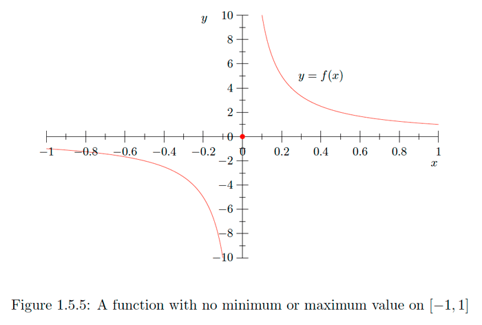
Let

\[f(x)=\left\{\begin{array}{ll}{\frac{1}{x},} & {\text { if }-1 \leq x<0 \text { or } 0<x \leq 1} , \\ {0,} & {\text { if } x=0.}\end{array}\right.\] See Figure \(1.5 .5 .\) Then \(f\) does not have a maximum value: if \(a \leq 0,\) then \(f(x)>f(a)\) for any \(x>0,\) and if \(a>0,\) then \(f(x)>f(a)\) whenever \(0<x<a\). Similarly, \(f\) has no minimum value: if \(a \geq 0,\) then \(f(x)<f(a)\) for any \(x<0\), and if \(a<0,\) then \(f(x)<f(a)\) whenever \(a<x<0 .\) The problem this time is that \(f\) is not continuous at \(x=0 .\) Indeed, if \(\epsilon\) is an infinitesimal, then \(f(\epsilon)\) is infinite, and, hence, not infinitesimally close to \(f(0)=0\).

Exercise \(\PageIndex{7}\)

Find an example of a continuous function which has both a minimum value and a maximum value on the open interval \((0,1)\).

Exercise \(\PageIndex{8}\)

Find an example of function which has a minimum value and a maximum value on the interval \([0,1],\) but is not continuous on \([0,1] .\)

The intermediate-value property states that a continuous function attains all values between any two given values of the function.

Theorem \(\PageIndex{12}\)

If \(f\) is continuous on the interval \([a, b]\) and \(m\) is any value betwen \(f(a)\) and \(f(b),\) then there exists a real number \(c\) in \([a, b]\) for which \(f(c)=m .\)

The next example shows that a function which is not continuous need not satisfy the intermediate-value property.

Example \(\PageIndex{10}\)

If \(H\) is the Heaviside function, then \(H(-1)=0\) and \(H(1)= 1\), but there does not exist any real number \(c\) in \([-1,1]\) for which \(H(c)=\frac{1}{2},\) even though \(0<\frac{1}{2}<1 .\)