1.10: Optimization

Optimization problems, that is, problems in which we seek to find the greatest or smallest value of some quantity, are common in the applications of mathematics. Because of the extreme-value property, there is a straightforward algorithm for solving optimization problems involving continuous functions on closed and bounded intervals. Hence we will treat this case first before considering functions on other intervals.

Recall that if \(f(c)\) is the maximum, or minimum, value of \(f\) on some interval \(I\) and \(f\) is differentiable at \(c,\) then \(f^{\prime}(c)=0 .\) Consequently, points at which the derivative vanishes will play an important role in our work on optimization.

Optimization on a Closed Interval

Suppose \(f\) is a continuous function on a closed and bounded interval \([a, b] .\) By the extreme-value property, \(f\) attains a maximum, as well as a minimum value, on \([a, b] .\) In particular, there is a real number \(c\) in \([a, b]\) such that \(f(c) \geq f(x)\) for all \(x\) in \([a, b] .\) If \(c\) in \((a, b)\) and \(f\) is differentiable at \(c,\) then we must have \(f^{\prime}(c)=0 .\) The only other possibilities are that \(f\) is not differentiable at \(c, c=a,\) or \(c=b .\) similar comments hold for points at which a minimum value occurs.

Definition: singular points

We call a real number \(c\) a singular point of a function \(f\) if \(f\) is defined on an open interval containing \(c,\) but is not differentiable at \(c .\)

Theorem \(\PageIndex{1}\)

If \(f\) is a continuous function on a closed and bounded interval \([a, b],\) then the maximum and minimum values of \(f\) occur at either

1. stationary points in the open interval \((a, b),
2. singular point in the open interval \((a, b),\) or ( 3) the endpoints of \([a, b] .\)

Hence we have the following procedure for optimizing a continuous function \(f\) on an interval \([a, b]:\)

1. Find all stationary and singular points of \(f\) in the open interval \((a, b)\).
2. Evaluate \(f\) at all stationary and singular points of \((a, b),\) and at the endpoints \(a\) and \(b .\)
3. The maximum value of \(f\) is the largest value found in step ( 2) and the minimum value of \(f\) is the smallest value found in step \((2) .\)

Example \(\PageIndex{1}\)

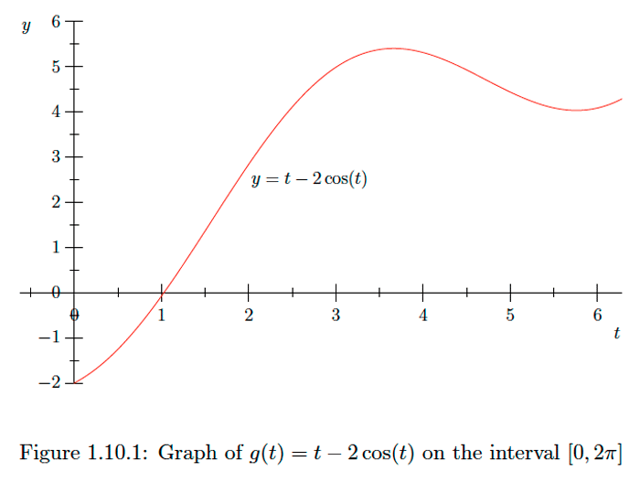
Consider the function \(g(t)=t-2 \cos (t)\) defined on the interval \([0,2 \pi] .\) Then

\[g^{\prime}(t)=1+2 \sin (t) ,\]

and so \(g^{\prime}(t)=0\) when

\[\sin (t)=-\frac{1}{2} .\]

For \(t\) in the open interval \((0,2 \pi),\) this means that either

\[t=\frac{7 \pi}{6}\]

or

\[t=\frac{11 \pi}{6} .\]

That is, the stationary points of \(g\) in \((0,2 \pi)\) are \(\frac{7 \pi}{6}\) and \(\frac{11 \pi}{6}\). Note that \(g\) is differentiable at all points in \((0,2 \pi),\) and so there are no singular points of \(g\) in \((0,2 \pi) .\) Hence to identify the extreme values of \(g\) we need evaluate only

\[g(0)=-2 ,\]

\[\begin{aligned} g\left(\frac{7 \pi}{6}\right) &=\frac{7 \pi}{6}+\sqrt{3} \approx 5.39724, \\ g\left(\frac{11 \pi}{6}\right) &=\frac{11 \pi}{6}-\sqrt{3} \approx 4.02753, \end{aligned}\]

and

\[g(2 \pi)=2 \pi-2 \approx 4.28319 .\]

Thus \(g\) has a maximum value of 5.39724 at \(t=\frac{7 \pi}{6}\) and a minimum value of \(-2\) at \(t=0 .\) See Figure 1.10 .1 for the graph of \(g\) on \([0,2 \pi] .\)

Exercise \(\PageIndex{1}\)

Find the maximum and minimum values of

\[f(x)=x^{2}+\frac{16}{x}\]

on the interval \([1,4]\).

Answer

Maximum value of 20 at \(x=4 ;\) minimum value of 12 at \(x=2\)

Exercise \(\PageIndex{2}\)

Find the maximum and minimum values of \(g(t)=t-\sin (2 t)\) on the interval \([0, \pi]\).

Answer

Maximum value of 3.4840 at \(t=\frac{5 \pi}{6} ;\) minimum value of \(-0.3424\) at \(t=\frac{\pi}{6}\)

Example \(\PageIndex{2}\)

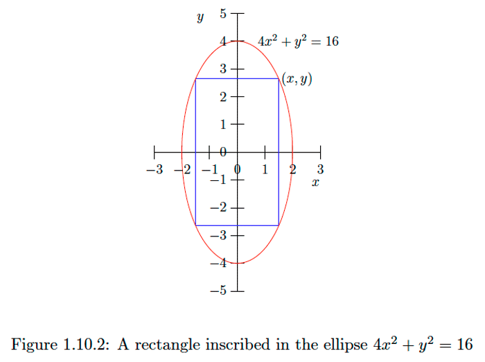
Suppose we inscribe a rectangle \(R\) inside the ellipse \(E\) with equation

\[4 x^{2}+y^{2}=16,\]

as shown in Figure \(1.10 .2 .\) If we let \((x, y)\) be the coordinates of the upper right-hand corner of \(R,\) then the area of \(R\) is

\[A=(2 x)(2 y)=4 x y.\]

since \((x, y)\) is a point on the upper half of the ellipse, we have

\[y=\sqrt{16-4 x^{2}}=2 \sqrt{4-x^{2}},\]

and so

\[A=8 x \sqrt{4-x^{2}}.\]

Now suppose we wish to find the dimensions of \(R\) which maximize its area. That is, we want to find the maximum value of \(A\) on the interval \([0,2] .\) Now

\[\frac{d A}{d x}=8 x \cdot \frac{-2 x}{2 \sqrt{4-x^{2}}}+8 \sqrt{4-x^{2}}=\frac{-8 x^{2}+8\left(4-x^{2}\right)}{\sqrt{4-x^{2}}}=\frac{32-16 x^{2}}{\sqrt{4-x^{2}}} .\]

Hence \(\frac{d A}{d x}=0,\) for \(x\) in \((0,2),\) when \(32-16 x^{2}=0,\) that is, when \(x=\sqrt{2} .\) Thus the maximum value of \(A\) must occur at \(x=0, x=\sqrt{2},\) or \(x=2 .\) Evaluating, we have

\[\left.A\right|_{x=0}=0,\]

\[\left.A\right|_{x=\sqrt{2}}=8 \sqrt{2} \sqrt{2}=16,\]

and

\[\left.A\right|_{x=2}=0.\]

Hence the rectangle \(R\) inscribed in \(E\) with the largest area has area 16 when \(x=\sqrt{2}\) and \(y=2 \sqrt{2} .\) That is, \(R\) is \(2 \sqrt{2}\) by \(4 \sqrt{2}\).

Exercise \(\PageIndex{3}\)

Find the dimensions of the rectangle \(R\) with largest area which may be inscribed in the ellipse with equation

\[\frac{x^{2}}{a^{2}}+\frac{y^{2}}{b^{2}}=1,\]

where \(a\) and \(b\) are positive real numbers.

Answer

\(R\) is \(\sqrt{2} a\) by \(\sqrt{2} b\)

Exercise \(\PageIndex{4}\)

A piece of wire, 100 centimeters in length, is cut into two pieces, one of which is used to form a square and the other a circle. Find the lengths of the pieces so that sum of the areas of the square and the circle are (a) maximum and (b) minimum.

Answer

(a) all the wire is used for the circle;

(b) 43.99 cm use for the square, \(56.01 \mathrm{cm}\) used for the circle

Exercise \(\PageIndex{5}\)

Show that of all rectangles of a given perimeter \(P,\) the square is the one with the largest area

Optimization on Other Intervals

We now consider the case of a continuous function \(f\) on an interval \(I\) which is either not closed or not bounded. The extreme-value property does not apply in this case, and, as we have seen, we have no guarantee that \(f\) has an extreme value on the interval. Hence, in general, this situation requires more careful analysis than that of the previous section.

However, there is one case which arises frequently and which is capable of a simple analysis. Suppose that \(c\) is a point in \(I\) which is either a stationary or singular point of \(f,\) and that \(f\) is differentiable at all other points of \(I\). If \(f^{\prime}(x)<0\) for all \(x\) in \(I\) with \(x<c\) and \(f^{\prime}(x)>0\) for all \(x\) in \(I\) with \(c<x,\) then \(f\) is decreasing before \(c\) and increasing after \(c,\) and so must have a minimum value at \(c .\) Similarly, if \(f^{\prime}(x)>0\) for all \(x\) in \(I\) with \(x<c\) and \(f^{\prime}(x)<0\) for all \(x\) in \(I\) with \(c<x,\) then \(f\) is increasing before \(c\) and decreasing after \(c,\) and so must have a maximum value at \(c .\) The next examples will illustrate.

Example \(\PageIndex{3}\)

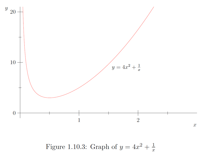
Consider the problem of finding the extreme values of

\[ y=4 x^{2}+\frac{1}{x} \]

on the interval \((0, \infty) .\) Since

\[\frac{d y}{d x}=8 x-\frac{1}{x^{2}} ,\]

we see that \(\frac{d y}{d x}<0\) when, and only when,

\[8 x<\frac{1}{x^{2}} .\]

This is equivalent to

\[x^{3}<\frac{1}{8} ,\]

so \(\frac{d y}{d x}<0\) on \((0, \infty)\) when, and only when, \(0<x<\frac{1}{2} .\) Similarly, we see that \(\frac{d y}{d x}>0\) when, and only when, \(x>\frac{1}{2} .\) Thus \(y\) is a decreasing function of \(x\) on the interval \(\left(0, \frac{1}{2}\right)\) and an increasing function of \(x\) on the interval \(\left(\frac{1}{2}, \infty\right),\) and so must have an minimum value at \(x=\frac{1}{2} .\) Note, however, that \(y\) does not have a maximum value: given any \(x=c,\) if \(c<\frac{1}{2}\) we may find a larger value for \(y\) by using any \(0<x<c,\) and if \(c>\frac{1}{2}\) we may find a larger value for \(y\) by using any \(x>c .\) Thus we conclude that \(y\) has a minimum value of 3 at \(x=\frac{1}{2},\) but does not have a maximum value. See Figure \(1.10 .3 .\)

Example \(\PageIndex{4}\)

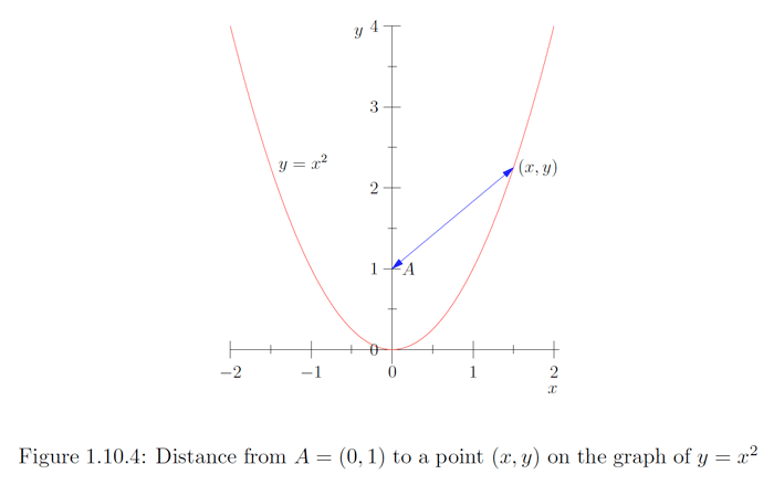
Consider the problem of finding the shortest distance from the point \(A=(0,1)\) to the parabola \(P\) with equation \(y=x^{2} .\) If \((x, y)\) is a point on \(P (\text { see Figure } 1.10 .4),\) then the distance from \(A\) to \((x, y)\) is

\[D=\sqrt{(x-0)^{2}+(y-1)^{2}}=\sqrt{x^{2}+\left(x^{2}-1\right)^{2}} .\]

Our problem then is to find the minimum value of \(D\) on the interval \((-\infty, \infty) .\) However, to make the problem somewhat easier to work with, we note that, since \(D\) is always a positive value, finding the minimum value of \(D\) is equivalent

to finding the minimum value of \(D^{2} .\) So letting

\[z=D^{2}=x^{2}+\left(x^{2}-1\right)^{2}=x^{2}+x^{4}-2 x^{2}+1=x^{4}-x^{2}+1 ,\]

our problem becomes that of finding the minimum value of \(z\) on \((-\infty, \infty) .\) Now

\[\frac{d z}{d x}=4 x^{3}-2 x ,\]

so \(\frac{d z}{d x}=0\) when, and only when,

\[0=4 x^{3}-2 x=2 x\left(2 x^{2}-1\right) ,\]

that is, when, and only when, \(x=-\frac{1}{\sqrt{2}}, x=0,\) or \(x=\frac{1}{\sqrt{2}} .\) Now \(2 x<0\) when \(-\infty<x<0\) and \(2 x>0\) when \(0<x<\infty,\) whereas \(2 x^{2}-1<0\) when \(-\frac{1}{\sqrt{2}}<x<\frac{1}{\sqrt{2}}\) and \(2 x^{2}-1>0\) either when \(x<-\frac{1}{\sqrt{2}}\) or when \(x>\frac{1}{\sqrt{2}} .\) Taking the product of \(2 x\) and \(2 x^{2}-1,\) we see that \(\frac{d z}{d x}<0\) when \(x<-\frac{1}{\sqrt{2}}\) and when \(0<x<\frac{1}{\sqrt{2}},\) and \(\frac{d z}{d x}>0\) when \(-\frac{1}{\sqrt{2}}<x<0\) and when \(x>\frac{1}{\sqrt{2}} .\) It follows that \(z\) is a decreasing function of \(x\) on \(\left(-\infty,-\frac{1}{\sqrt{2}}\right)\) and on \(\left(0, \frac{1}{\sqrt{2}}\right),\) and is an increasing function of \(x\) on \(\left(-\frac{1}{\sqrt{2}}, 0\right)\) and on \(\left(\frac{1}{\sqrt{2}}, \infty\right)\).

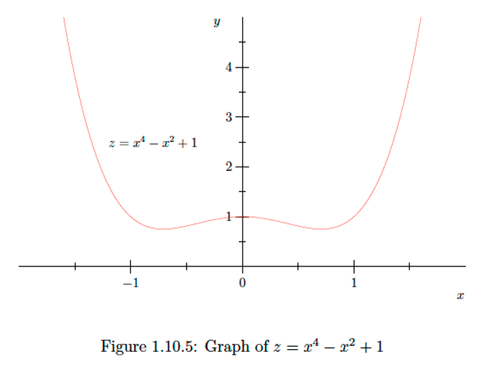
It now follows that \(z\) has a local minimum of \(\frac{3}{4}\) at \(x=-\frac{1}{\sqrt{2}},\) a local maximum of 1 at \(x=0,\) and another local minimum of \(\frac{3}{4}\) at \(x=\frac{1}{\sqrt{2}} .\) Note that \(\frac{3}{4}\) is the minimum value of \(z\) both on the the interval \((-\infty, 0)\) and on the interval \((0, \infty) ;\) since \(z\) has a local maximum of 1 at \(x=0,\) it follows that \(\frac{3}{4}\) is in fact the minimum value of \(z\) on \((-\infty, \infty) .\) Hence we may conclude that the minimum distance from \(A\) to \(P\) is \(\frac{\sqrt{3}}{2},\) and the points on \(P\) closest to \(A\) are \(\left(-\frac{1}{\sqrt{2}}, \frac{1}{2}\right)\) and \(\left(\frac{1}{\sqrt{2}}, \frac{1}{2}\right) .\) Note, however, that \(z\) does not have a maximum value, even though it has a local maximum value at \(x=0 .\) See Figure 1.10 .5 for the graph of \(z\).

Exercise \(\PageIndex{6}\)

Find the point on the parabola \(y=x^{2}\) which is closest to the point \((3,0)\).

Answer

\((1,1)\)

Exercise \(\PageIndex{7}\)

Show that of all rectangles of a given area \(A,\) the square is the one with the shortest perimeter.

Exercise \(\PageIndex{8}\)

Show that of all right circular cylinders with a fixed volume \(V,\) the one with height and diameter equal has the minimum surface area.

Exercise \(\PageIndex{9}\)

Find the points on the ellipse \(4 x^{2}+y^{2}=16\) which are \((a)\) closest to and (b) farthest from the point \((0,1)\).

Answer

(a) \(\left(\frac{4 \sqrt{2}}{3}, \frac{4}{3}\right)\) and \(\left(-\frac{4 \sqrt{2}}{3}, \frac{4}{3}\right)\) (b) \((0,-4)\)