
1.9: Increasing, Decreasing, and Local Extrema
- Page ID
- 25430

( \newcommand{\kernel}{\mathrm{null}\,}\)
Recall that the slope of a line is positive if, and only if, the line rises from left to right. That is, if m>0,f(x)=mx+b, and u<v, then
f(v)=mv+b=mv−mu+mu+b=m(v−u)+mu+b>mu+b=f(u).The Mean-Value Theorem
Recall that the extreme value property tells us that a continuous function on a closed interval must attain both a minimum and a maximum value. Suppose f is continuous on [a,b], differentiable on (a,b), and f attains a maximum value at c with a<c<b. In particular, for any infinitesimal dx,f(c)≥f(c+dx), and so, equivalently, f(c+dx)−f(c)≤0. It follows that if dx>0,
f(c+dx)−f(c)dx≤0,Theorem 1.9.1
If f is differentiable on (a,b) and attains a maximum, or a minimum, value at c, then f′(c)=0.
Now suppose f is continuous on [a,b], differentiable on (a,b), and f(a)=f(b). If f is a constant function, then f′(c)=0 for all c in (a,b). If f is not constant, then there is a point c in (a,b) at which f attains either a maximum or a minimum value, and so f′(c)=0. In either case, we have the following result, known as Rolle's theorem.
Theorem 1.9.2
If f is continuous on [a,b], differentiable on (a,b), and f(a)=f(b), then there is a real number c in (a,b) for which f′(c)=0.
More generally, suppose f is continuous on [a,b] and differentiable on (a,b).
Let g(x)=f(x)−f(b)−f(a)b−a(x−a)−f(a).so we must have
0=g′(c)=f′(c)−f(b)−f(a)b−a.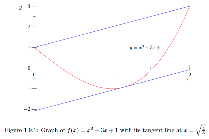
Theorem 1.9.3
If f is continuous on [a,b] and differentiable on (a,b), then there exists a real number c in (a,b) for which
f′(c)=f(b)−f(a))b−a.Example 1.9.1
Consider the function f(x)=x3−3x+1 on the interval [0,2]. By the mean-value theorem, there must exist at least one point c in [0,2] for which
f′(c)=f(2)−f(0)2−0=3−12=1.Increasing and Decreasing Functions
The preceding discussion leads us to the following definition and theorem.
Definition
We say a function f is increasing on an interval I if, whenever a<b are points in I,f(a)<f(b). Similarly, we say f is decreasing on I if, whenever a<b are points in I,f(a)>f(b).
Now suppose f is a defined on an interval I and f′(x)>0 for every x in I which is not an endpoint of I. Then given any a and b in I, by the mean-value theorem there exists a point c between a and b for which
f(b)−f(a)b−a=f′(c)>0.Theorem 1.9.4
Suppose f is defined on an interval I. If f′(x)>0 for every x in I which is not an endpoint of I, then f is increasing on I. If f′(x)<0 for every x in I which is not an endpoint of I, then f is decreasing on I.
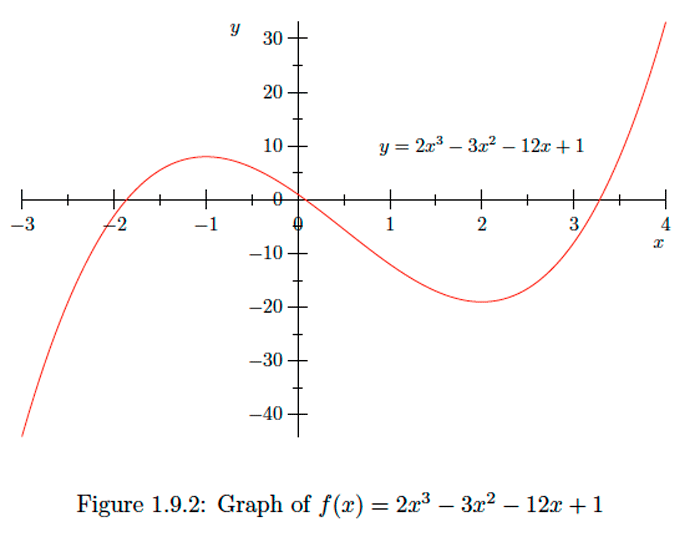
Example 1.9.2
Let f(x)=2x3−3x2−12x+1. Then
f′(x)=6x2−6x−12=6(x2−x−2)=6(x−2)(x+1).Definition
We say f has a local marimum at a point c if there exists an interval (a,b) containing c for which f(c)≥f(x) for all x in (a,b). Similarly, we say f has a local minimum at a point c if there exists an interval (a,b) containing c for which f(c)≤f(x) for all x in (a,b). We say f has a local extremum at c if f has either a local maximum or a local minimum at c.
We may now rephrase Theorem 1.9 .1 as follows.
Theorem 1.9.5
If f is differentiable at c and has a local extremum at c, then f′(c)=0.
As illustrated in the preceding example, we may identify local minimums of a function f by locating those points at which f changes from decreasing to increasing, and local maximums by locating those points at which f changes from increasing to decreasing.
Example 1.9.3
Let f(x)=x+2sin(x). Then f′(x)=1+2cos(x), and so f′(x)<0 when, and only when,
cos(x)<−12.n=0,±1,±2,… It now follows that f has a local maximum at every point of the form
x=2π3+2πn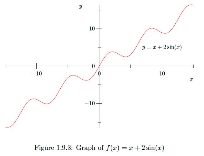
Exercise 1.9.1
Find the intervals where f(x)=x3−6x is increasing and the intervals where f is decreasing. Use this information to identify any local maximums or local minimums of f.
- Answer
-
f is increasing on (−∞,−√2) and on [√2,∞], decreasing on [−√2,√2]; f has a local maximum of 4√2 at x=−√2 and a local minimum of −4√2 at x=√2.
Exercise 1.9.2
Find the intervals where f(x)=5x3−3x5 is increasing and the intervals where f is decreasing. Use this information to identify any local maximums or local minimums of f.
- Answer
-
f is increasing on [−1,0] and on [0,1] (or, simply, [−1,1];f is decreasing on (−∞,−1] and on [1,∞);f has a local maximum of 2 at x=1 and a local minimum of −2 at x=−1.
Exercise 1.9.3
Find the intervals where f(x)=x+sin(x) is increasing and the intervals where f is decreasing. Use this information to identify any local maximums or local minimums f.
- Answer
-
f is increasing on all intervals of the form [−nπ,nπ], where n=1,2,…; f has no local maximums or minimums (indeed, f is increasing on (−∞,∞)).