4.9: Inverse Trigonometric Functions

The trigonometric functions frequently arise in problems, and often it is necessary to invert the functions, for example, to find an angle with a specified sine. Of course, there are many angles with the same sine, so the sine function doesn't actually have an inverse that reliably "undoes'' the sine function. If you know that \(\sin x=0.5\), you can't reverse this to discover \(x\), that is, you can't solve for \(x\), as there are infinitely many angles with sine \(0.5\). Nevertheless, it is useful to have something like an inverse to the sine, however imperfect. The usual approach is to pick out some collection of angles that produce all possible values of the sine exactly once. If we "discard'' all other angles, the resulting function does have a proper inverse.

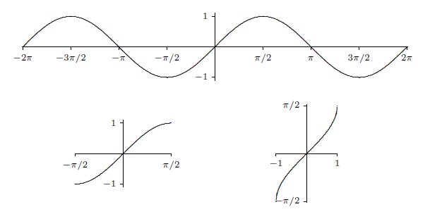
The sine takes on all values between \(-1\) and \(1\) exactly once on the interval \([-\pi/2,\pi/2]\). If we truncate the sine, keeping only the interval \([-\pi/2,\pi/2]\), as shown in figure 4.9.1, then this truncated sine has an inverse function. We call this the inverse sine or the arcsine, and write \(y=\arcsin(x)\).

Figure 4.9.1. The sine, the truncated sine, the inverse sine.

Recall that a function and its inverse undo each other in either order, for example, \( (\root3\of x)^3=x\) and \( \root3\of{x^3}=x\). This does not work with the sine and the "inverse sine'' because the inverse sine is the inverse of the truncated sine function, not the real sine function. It is true that \(\sin(\arcsin(x))=x\), that is, the sine undoes the arcsine.

It is not true that the arcsine undoes the sine, for example, \(\sin(5\pi/6)=1/2\) and \(\arcsin(1/2)=\pi/6\), so doing first the sine then the arcsine does not get us back where we started. This is because \(5\pi/6\) is not in the domain of the truncated sine. If we start with an angle between \(-\pi/2\) and \(\pi/2\) then the arcsine does reverse the sine: \(\sin(\pi/6)=1/2\) and \(\arcsin(1/2)=\pi/6\).

What is the derivative of the arcsine? Since this is an inverse function, we can discover the derivative by using implicit differentiation. Suppose \(y=\arcsin(x)\). Then \[\sin(y)=\sin(\arcsin(x))=x.\] Now taking the derivative of both sides, we get

\[\eqalign{ y'\cos y &= 1\cr y'={1\over \cos y}\cr }\]

As we expect when using implicit differentiation, \(y\) appears on the right hand side here. We would certainly prefer to have \(y'\) written in terms of \(x\), and as in the case of \(\ln x\) we can actually do that here. Since \( \sin^2y+\cos^2 y=1\), \( \cos^2y=1-\sin^2y=1-x^2\). So \( \cos y=\pm\sqrt{1-x^2 }\), but which is it---plus or minus? It could in general be either, but this isn't "in general'': since \(y=\arcsin(x)\) we know that \(-\pi/2\le y\le \pi/2\), and the cosine of an angle in this interval is always positive. Thus

\[ \cos y=\sqrt{1-x^2 }\]

and

\[{d\over dx}\arcsin(x)={1\over \sqrt{1-x^2 }}.\]

Note that this agrees with figure 4.9.1: the graph of the arcsine has positive slope everywhere.

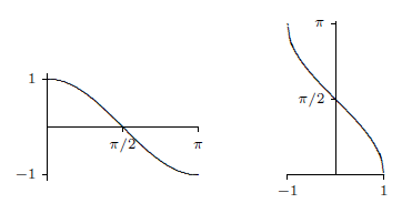
We can do something similar for the cosine. As with the sine, we must first truncate the cosine so that it can be inverted, as shown in figure 4.9.2. Then we use implicit differentiation to find that

\[{d\over dx}\arccos(x)={-1\over \sqrt{1-x^2 }}.\]

Note that the truncated cosine uses a different interval than the truncated sine, so that if \(y=\arccos(x)\) we know that \(0\le y\le \pi\). The computation of the derivative of the arccosine is left as an exercise.

Figure 4.9.2. The truncated cosine, the inverse cosine.

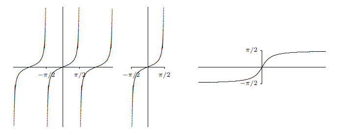
Finally we look at the tangent; the other trigonometric functions also have "partial inverses'' but the sine, cosine and tangent are enough for most purposes. The tangent, truncated tangent and inverse tangent are shown in figure 4.9.3; the derivative of the arctangent is left as an exercise.

Figure 4.9.3. The tangent, the truncated tangent, the inverse tangent.

Contributors

David Guichard (Whitman College)

• Integrated by Justin Marshall.