9.4: Average Value of a Function

The average of some finite set of values is a familiar concept. If, for example, the class scores on a quiz are 10, 9, 10, 8, 7, 5, 7, 6, 3, 2, 7, 8, then the average score is the sum of these numbers divided by the size of the class: $$\hbox{average score} = {10+ 9+ 10+ 8+ 7+ 5+ 7+ 6+ 3+ 2+ 7+ 8\over 12}={82\over 12}\approx 6.83. \nonumber$$ Suppose that between $t=0$ and $t=1$ the speed of an object is $\sin(\pi t)$. What is the average speed of the object over that time? The question sounds as if it must make sense, yet we can't merely add up some number of speeds and divide, since the speed is changing continuously over the time interval.

To make sense of "average'' in this context, we fall back on the idea of approximation. Consider the speed of the object at tenth of a second intervals: $\sin 0$, $\sin(0.1\pi)$, $\sin(0.2\pi)$, $\sin(0.3\pi)$,…, $\sin(0.9\pi)$. The average speed "should'' be fairly close to the average of these ten speeds: $${1\over 10}\sum_{i=0}^9 \sin(\pi i/10)\approx {1\over 10}6.3=0.63. \nonumber$$Of course, if we compute more speeds at more times, the average of these speeds should be closer to the "real'' average. If we take the average of $n$ speeds at evenly spaced times, we get: $${1\over n} \sum_{i=0}^{n-1} \sin(\pi i/n). \nonumber$$\ Here the individual times are $t_i=i/n$, so rewriting slightly we have $${1\over n}\sum_{i=0}^{n-1} \sin(\pi t_i). \nonumber$$This is almost the sort of sum that we know turns into an integral; what's apparently missing is $\Delta t$---but in fact, $\Delta t=1/n$, the length of each subinterval. So rewriting again: $$\sum_{i=0}^{n-1} \sin(\pi t_i){1\over n}= \sum_{i=0}^{n-1} \sin(\pi t_i)\Delta t. \nonumber$$Now this has exactly the right form, so that in the limit we get $$\hbox{average speed} = \int_0^1 \sin(\pi t)\,dt= \left.-{\cos(\pi t)\over\pi}\right|_0^1= -{\cos(\pi)\over \pi}+{\cos(0)\over\pi}={2\over\pi}\approx 0.6366\approx 0.64. \nonumber$$

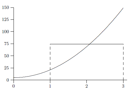
It's not entirely obvious from this one simple example how to compute such an average in general. Let's look at a somewhat more complicated case. Suppose that the velocity of an object is $16 t^2+5$ feet per second. What is the average velocity between $t=1$ and $t=3$? Again we set up an approximation to the average: $${1\over n}\sum_{i=0}^{n-1} 16t_i^2+5, \nonumber$$where the values $t_i$ are evenly spaced times between 1 and 3. Once again we are "missing'' $\Delta t$, and this time $1/n$ is not the correct value. What is $\Delta t$ in general? It is the length of a subinterval; in this case we take the interval $[1,3]$ and divide it into $n$ subintervals, so each has length $(3-1)/n=2/n=\Delta t$. Now with the usual "multiply and divide by the same thing'' trick we can rewrite the sum: $${1\over n}\sum_{i=0}^{n-1} 16t_i^2+5= {1\over 3-1}\sum_{i=0}^{n-1} (16t_i^2+5){3-1\over n}= {1\over 2}\sum_{i=0}^{n-1} (16t_i^2+5){2\over n}= {1\over 2}\sum_{i=0}^{n-1} (16t_i^2+5)\Delta t. \nonumber$$In the limit this becomes $${1\over 2}\int_1^3 16t^2+5\,dt={1\over 2}{446\over 3}={223\over 3}. \nonumber$$Does this seem reasonable? Let's picture it: in figure 9.4.1 is the velocity function together with the horizontal line $y=223/3\approx 74.3$. Certainly the height of the horizontal line looks at least plausible for the average height of the curve.

Figure 9.4.1. Average velocity.

Here's another way to interpret "average'' that may make our computation appear even more reasonable. The object of our example goes a certain distance between $t=1$ and $t=3$. If instead the object were to travel at the average speed over the same time, it should go the same distance. At an average speed of $223/3$ feet per second for two seconds the object would go $446/3$ feet. How far does it actually go? We know how to compute this: $$\int_1^3 v(t)\,dt = \int_1^3 16t^2+5\,dt={446\over 3}. \nonumber$$So now we see that another interpretation of the calculation $${1\over 2}\int_1^3 16t^2+5\,dt={1\over 2}{446\over 3}={223\over 3} \nonumber$$is: total distance traveled divided by the time in transit, namely, the usual interpretation of average speed.

In the case of speed, or more properly velocity, we can always interpret "average'' as total (net) distance divided by time. But in the case of a different sort of quantity this interpretation does not obviously apply, while the approximation approach always does. We might interpret the same problem geometrically: what is the average height of $16x^2+5$ on the interval $[1,3]$? We approximate this in exactly the same way, by adding up many sample heights and dividing by the number of samples. In the limit we get the same result: $$\lim_{n\to\infty}{1\over n}\sum_{i=0}^{n-1} 16x_i^2+5= {1\over 2}\int_1^3 16x^2+5\,dx={1\over 2}{446\over 3}={223\over 3}. \nonumber$$We can interpret this result in a slightly different way. The area under $y=16x^2+5$ above $[1,3]$ is $$\int_1^3 16t^2+5\,dt={446\over 3}. \nonumber$$The area under $y=223/3$ over the same interval $[1,3]$ is simply the area of a rectangle that is 2 by $223/3$ with area $446/3$. So the average height of a function is the height of the horizontal line that produces the same area over the given interval.

Contributors and Attributions

• David Guichard (Whitman College)

• Integrated by Justin Marshall.