15.2: Double Integrals in Cylindrical Coordinates

Suppose we have a surface given in cylindrical coordinates as \(z=f(r,\theta)\) and we wish to find the integral over some region. We could attempt to translate into rectangular coordinates and do the integration there, but it is often easier to stay in cylindrical coordinates.

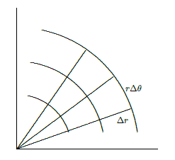
How might we approximate the volume under such a surface in a way that uses cylindrical coordinates directly? The basic idea is the same as before: we divide the region into many small regions, multiply the area of each small region by the height of the surface somewhere in that little region, and add them up. What changes is the shape of the small regions; in order to have a nice representation in terms of \(r\) and \(\theta\), we use small pieces of ring-shaped areas, as shown in Figure \(\PageIndex{1}\). Each small region is roughly rectangular, except that two sides are segments of a circle and the other two sides are not quite parallel. Near a point \((r,\theta)\), the length of either circular arc is about \(r\Delta\theta\) and the length of each straight side is simply \(\Delta r\). When \(\Delta r\) and \(\Delta \theta\) are very small, the region is nearly a rectangle with area \(r\Delta r\Delta\theta\), and the volume under the surface is approximately

\[\sum\sum f(r_i,\theta_j)r_i\Delta r\Delta\theta.\]

In the limit, this turns into a double integral \[\int_{\theta_0}^{\theta_1}\int_{r_0}^{r_1} f(r,\theta)r\,dr\,d\theta.\]

Figure \(\PageIndex{1}\): A cylindrical coordinate "grid".

Example \(\PageIndex{1}\)

Find the volume under \(z=\sqrt{4-r^2}\) above the quarter circle bounded by the two axes and the circle \(x^2+y^2=4\) in the first quadrant.

Solution

In terms of \(r\) and \(\theta\), this region is described by the restrictions \(0\le r\le 2\) and \(0\le\theta\le\pi/2\), so we have

\[\eqalign{
\int_{0}^{\pi/2}\int_{0}^{2} \sqrt{4-r^2}\;r\,dr\,d\theta
&=\int_{0}^{\pi/2}\left. -{1\over3}(4-r^2)^{3/2}\right|_0^2\,d\theta\cr
&=\int_{0}^{\pi/2} {8\over3}\,d\theta\cr
&={4\pi\over3}.\cr
}\]

The surface is a portion of the sphere of radius 2 centered at the origin, in fact exactly one-eighth of the sphere. We know the formula for volume of a sphere is \((4/3)\pi r^3\), so the volume we have computed is \((1/8)(4/3)\pi 2^3=(4/3)\pi\), in agreement with our answer.

This example is much like a simple one in rectangular coordinates: the region of interest may be described exactly by a constant range for each of the variables. As with rectangular coordinates, we can adapt the method to deal with more complicated regions.

Example \(\PageIndex{2}\)

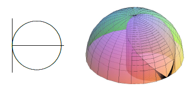
Find the volume under \(z=\sqrt{4-r^2}\) above the region enclosed by the curve \(r=2\cos\theta\), \(-\pi/2\le\theta\le\pi/2\); see figure \(\PageIndex{2}\).

Figure \(\PageIndex{2}\): Volume over a region with non-constant limits.

Solution

The region is described in polar coordinates by the inequalities \(-\pi/2\le\theta\le\pi/2\) and \(0\le r\le2\cos\theta\), so the double integral is

\[
\int_{-\pi/2}^{\pi/2}\int_{0}^{2\cos\theta} \sqrt{4-r^2}\;r\,dr\,d\theta
=2\int_{0}^{\pi/2}\int_{0}^{2\cos\theta} \sqrt{4-r^2}\;r\,dr\,d\theta.
\]

We can rewrite the integral as shown because of the symmetry of the volume; this avoids a complication during the evaluation. Proceeding:

\[\eqalign{
2\int_{0}^{\pi/2}\int_{0}^{2\cos\theta} \sqrt{4-r^2}\;r\,dr\,d\theta
&=2\int_{0}^{\pi/2}-{1\over3}\left.(4-r^2)^{3/2}\right|_0^{2\cos\theta}\,d\theta\cr
&=2\int_{0}^{\pi/2}-{8\over3}\sin^3\theta+{8\over3}\,d\theta\cr
&=\left.2\left(-{8\over3}{\cos^3\theta\over3}-\cos\theta+{8\over3}\theta\right)\right|_0^{\pi/2}\cr
&={8\over3}\pi-{32\over9}.\cr
}\]

You might have learned a formula for computing areas in polar coordinates. It is possible to compute areas as volumes, so that you need only remember one technique. Consider the surface \(z=1\), a horizontal plane. The volume under this surface and above a region in the \(x\)-\(y\) plane is simply \(1\cdot(\hbox{area of the region})\), so computing the volume really just computes the area of the region.

Example \(\PageIndex{3}\)

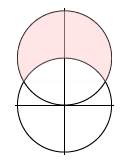
Find the area outside the circle \(r=2\) and inside \(r=4\sin\theta\); see Figure \(\PageIndex{3}\).

Figure 15.2.3. Finding are by computing volume.

Solution

The region is described by \(\pi/6\le\theta\le5\pi/6\) and \(2\le r\le4\sin\theta\), so the integral is

\[\eqalign{
\int_{\pi/6}^{5\pi/6}\int_2^{4\sin\theta}1\,r\,dr\,d\theta
&=\int_{\pi/6}^{5\pi/6}\left. {1\over2}r^2\right|_2^{4\sin\theta}\,d\theta\cr
&=\int_{\pi/6}^{5\pi/6}8\sin^2\theta-2\,d\theta\cr
&={4\over3}\pi+2\sqrt3.\cr
}\]

Contributors

• David Guichard (Whitman College)

• Integrated by Justin Marshall.